Dome at Cold Revisited

There were 4 dome teams playing in wintery weather today, and all four lost. DET lost at PHI, MIN lost at BAL, IND lost at CIN, and ATL lost at GB.

A few years ago I looked at how dome teams tend to struggle in cold weather. I wanted to know if dome team underperformance in the cold was indeed true and if so how big was the effect. The answers were: Yes and huge. Last season I redid things using actual game temperatures and found just as big an effect.

With the weather as it is on the east coast today, I looked at this phenomenon once again. We have two more years worth of data thanks to the addition of 1999. Plus, I was able to reconstruct nearly another half season worth of data by replacing missing game temperatures from the gamebooks. I also broke out teams that played in retractable-roof stadiums by season.

Here are the results if we count retractable teams as dome teams. There's a case to be made that retractable home environments are closer to dome environments than open air stadiums. The chart below plots road team winning percentage according to game temperature.

Rest vs. Rust After Thursday Night Football

Andrew Mooney is the Co-President of the Harvard Sports Analysis Collective. He is a senior majoring in Social Studies, which is another way of saying he's an economics major. Andrew has worked as an analytics intern in the NFL for about two years, and previously wrote for the Stats Driven blog at Boston.com. He's a big fan of all Detroit sports, and he'll throw an octopus on your ice if you're not watching.

In struggling out of my bed at the witching hour of 8:00 am this morning, I had to wonder how much more equipped to tackle the day’s challenges I would be with an hour more of sleep. I then noticed that I wasn’t missing the tip of my finger, nor had I sustained a concussion the day before, incidents from which I would need significantly more than a week to recover. In this state of empathy, I couldn’t think of a more welcome time of the NFL season for a player than an extra day or two off.

Though I’m sure it provides players some much needed rest, it is not immediately clear what effect this time off has on performance. The qualitative cases for each side are pretty straightforward, and your grandfather used each of them liberally in instructing you in the wonders of sporting conventional wisdom. “Ah, they had an extra week to prepare AND get healthy,” he said knowingly after Washington’s 31-6 thrashing of the Eagles last season. “They just got rusty,” he told you after the Vikings fell to Chicago, 28-10, the following week. “What in the Sam Hill…” he muttered after the 49ers and Rams battled to a 24-24 tie.

Washington Post: All About Home Field Advantage

Following a Redskins win that broke an eight-game home losing streak, this week's article at the Post looks at home field advantage and its causes.

Home advantage is universal in sports. Whether it’s a team or individual sport, professional or amateur, virtually all athletic competitions have a home advantage. Fans like to believe they are the cause. Communication is essential in football, audibles and snap counts being the most obvious. The players themselves tell us it makes a difference. As plausible as this explanation may seem, the evidence suggests home advantage does not come from the crowd.

Home Field Advantage Is Not Out of Whack So Far

I've seen a number of articles about how NFL home field advantage has been very strong in terms of home and visitor scores. The thinking is that the replacement refs may be more influenced by home crowds than their more experienced predecessors. While I can't rule out that possibility, I can say it's premature to definitively say one way or another.

In week 1 the average HFA was 3.2 net points, and in week 2 it was 8.7 net points. As I write, Week 3's average is -1.9 net points through 14 games. Week 1 was obviously well within the long term trend of 2.5 net points for the home team, and Week 3 tilted slightly toward the visitors. But week 2 showed a large advantage for home teams. We know there is week-to-week variance in net scores for home teams, but how far from ordinary is 8.7 net points for the home team in a single week?

Since 2000 the standard deviation for weekly average HFA is 4.0 points, and the average is 2.4 points, which means week 2's 8.7 is not 2 standard deviations from the mean (p=0.40). Week 2 featured only the 15th largest HFA in the past 12+ years. The regular refs were on the field for the 14 weeks with larger HFAs.

The chart below shows the distribution of weekly average HFA in net points for the home team.

Hawks, Doves, and Home Field Advantage

Sports researchers have been studying home field advantage for decades. It’s a universal phenomenon found in virtually every sport, and professional football is no exception. Home teams win 57% of all regular season games in the NFL. Measuring it is easy. The question is, what causes it?

Several studies have tested theories about crowd noise, referee bias, time zone effects, climate, and peculiarties of ballparks. But these effects have not been shown to account for much if any of HFA.

Some recent research looked at when HFA manifests itself in games. In the NBA, HFA (or HCA rather)  is strongest in the beginning of the game and then diminishes as it goes on. I found the same phenomenon in the NFL. The first quarter shows the strongest HFA by far. Now, baseball research reveals the same phenomenon. It’s also been shown that HFA in the NFL is strongest between inter-conference games and weaker between intra-divisional games. With the advent of inter-league play, baseball also appears to have the same tendency.

I think these findings all point toward the same theory, namely that a significant portion of HFA comes from environmental familiarity. I’m not talking about the quirks of an outfield or the type of turf in a stadium. I’m talking about the whole picture—the way we all feel comfortable when we’re in familiar surroundings and often feel anxious in strange places.

I think that game theory can help explain why this is the case. I’m not referring to the usual run-pass or fastball-curve game theory we talk about in sports. Instead, I’m talking about natural selection and behavioral evolution. I realize this sounds a little out-there, but bear with me.

In-Game Home Field Advantage

Last season I discovered something interesting about home field advantage (HFA) in NFL games. It decreases as the game goes on. In terms of points scored by quarter, home teams have the biggest advantage in the 1st quarter, and then their advantage disappears by the end of the game. By the end of regulation, home teams and visiting teams perform equally well.

Although it’s clear that home teams perform better during a game, at least in terms of points scored, it’s not clear exactly how this translates into an increased chance of winning minute by minute. From simple win-loss records, all we know that at the outset of a game the home generally team ultimately has about a 56.5% chance of winning.

So there are (at least) two mechanisms at work. First is the decrease in performance advantage for the home team as the game goes on that I discussed above. Perhaps fatigue neutralizes the home team's edge, or perhaps it's visitor acclimation to a hostile, unfamiliar environment. Second, as the game clock ticks down, there is less time for the home team to capitalize on its advantage. By the end of the game the scoreboard doesn’t care which team is the home team and which is the visitor. A 1-point lead is good enough to win, period. So it’s a complicated thing to model. We just can’t add 6.5% to the win probability (WP) for the home team throughout the game.

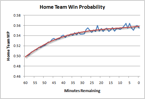
But I think I’ve cracked it. Using the WP model, which does not consider HFA, I can chart the average probability that the home team will win as the game goes on. It begins at 50% and by the end of the game it’s 56.5% (which I'll call a "6.5%" advantage).


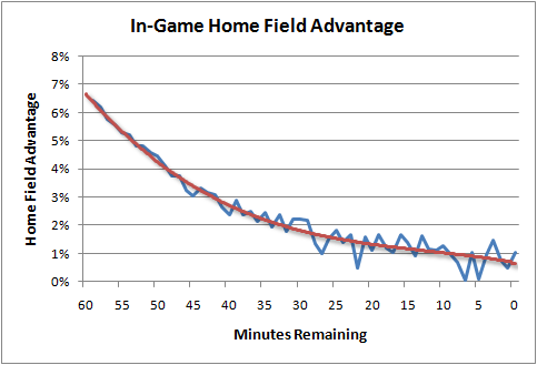
But we know that 6.5% advantage really exists as early as the first kickoff. It’s just that the model is “learning” and discovering that advantage as it actually accrues over the course of the game. So the shape of that curve is the shape of the curve of actual HFA, just in reverse.

Starting with a 6.5% advantage at kickoff, and following the shape of the curve, we see the real, no kidding, actual HFA as the game goes on. This isn’t HFA in terms of yards per play, first downs, or points scored, or in terms of anything except the probability of winning.


The HFA equation is:

%HFA = (-4E-05)t³ + 0.0056t² - 0.304t + 6.98

Where t is the time in minutes remaining in a game.

This now enables me to feed the strength of the advantage back into the win probability model to properly adjust for HFA. I would have to adjust the home field-agnostic WP with these values logistically (using the log of the odds ratios). This is because HFA would decrease in importance as one team or the other builds a large lead. HFA doesn’t really matter if a team has a 28-0 lead at halftime.

I've intended to include HFA into the WP model for a while, but just didn't know exactly how it declined through the course of the game. Now I know. Thanks to Ian for an insightful comment that got my wheels turning.

Weekly Roundup

Sabermetric Research points to this King Kaufman column in Salon.com. Kaufman takes sports writers to task for not appreciating advanced statistics. Sports writers and even some coaches are often dismissive of stats, and some even wear their ignorance as a badge of honor. Baseball is going through a quiet transformation based on advanced statistics. Stats are the cutting edge of the sport, and writers would do well to get on board. The way I see it, statistics is just a tool for learning from large sets of facts. Everyone relies on statistics one way or another. You can chose to do it well or do it poorly. Judging from the interest in this site and others, there is a sizable audience hungry for something other than the same old tired storylines we get from columnists and analysts.

Game theory could help improve the overtime problems in the NFL. This article talks about how to fairly divide something between two people. One of the best solutions is the I'll cut you choose method. So if two people splitting a piece of cake, one person would cut it in half, and the other picks which half he wants. The person cutting has an interest in making the division as fair as possible. Overtime could work the same way. The coin flip winner picks the yard line for kickoff, and the other team gets to chose whether to receive or kick. I don't think most traditionalists would like this idea, but neither team could complain about the outcome.

ZEUS chimes in on the Titans' decision to tie Ravens with a field goal instead of go for the first down on 4th and inches. Here was my take. But let me skip to the last chapter for everybody. It is almost always better to go for the first down, even up to 4th and 7 on a team's own side of the field in most cases. About the only times an NFL team should kick are on 4th and very long, or if time is expiring and the kick will win or tie the game.

ZEUS also thinks Coughlin was right to go for it against the Eagles. One thing about ZEUS, though--From what I can tell, the software is a simulation-based model. This means that it takes the current state of a game including score, time, field position, etc. and randomly simulates a game from that point forward. It does this 'millions' of times to estimate average win probabilities (that it calls game winning chance--GWC).

To me, this approach is fraught with problems. You'd have to model so many things so precisely to get a reliable result. The distributions of all possible play results for all the possible combinations of cirmcumstances simply could not be modeled with any reliability. You'd need to make a lot of assumptions, and the results are going to be very sensitive to those assumptions. It wouldn't be much different than playing out a game on Madden in auto-computer mode a million times. It just depends on the fidelity of the simulation. On the other hand, the advantage of this approach is that you can tweak the distributions to reflect specific team strengths and weaknesses.

Individual team abilities are mitigating considerations in kick or go-for-it decisions, but my take is that these factors are often overstated. Take the Ravens-Titans game. As I pointed out earlier this week, Baltimore had only scored on 2 of 10 possessions up until Fisher's decision to kick. That might indicate that the Titans defense could almost certainly count on stopping the Ravens offense. But the NFL average is 3 scores every 9 drives, not significantly different from 2 out of 10, and Baltimore went on to score to make it 3 out of 11. How much does under- or over-performance within a game predict performance later in a game? PFR took up that question and finds only about 25% of a team's under-performance in the first 3 quarters carries through to the 4th quarter.

Home field advantage (HFA) has been a focus of sports science for decades. We can quantify the strength of its effect pretty easily, but what are the causes? Is it travel fatigue, time zone change, weather, crowd noise, the shape of the field or cut of the grass, or referee bias? I think we now have pretty solid evidence that a large part of HFA comes from environmental familiarity.

The possible effect of general unfamiliarity was summed up well by a commenter: "From a psychological standpoint, performance could be subtlety infuenced due to players being in a somewhat unfamiliar environment due the small but cumulative effects of orienting to the new environment. This could be many things— the locker room, where the sun comes in over the stadium, the overall “feel.” All of these small distractions could influence performance–a performance that involves instantaneous decision making and physical reaction times. Research has shown that orienting to even environments that are somewhat unfamiliar influence memory, judgment, decison making, etc."

PFR took a look at HFA when opponents are familiar with each other. I thought that this might be what explains why HFA diminishes throughout a game. My suggestion was that because visitors are more familiar with environments when playing divisional opponents than when playing other opponents, we should see a reduced effect. And sure enough, that's exactly what we see. Division rivals not only have a reduced overall HFA, the quarter-by-quarter decline in HFA is shallower. To me, this is evidence that a good deal of HFA in the NFL is due to overall environmental familiarity. I think this is very interesting, and it comes mostly from loose collaboration from people who've never met. Twenty years ago, before the internet, research like this wouldn't be possible. We're not curing cancer, but it is interesting and useful. Further comments here.

Smart Football dissects the deep crossing route.

The Numbers Guy takes a look at rare NFL scores. The Chargers-Steelers 11-10 score is not the only unique score this year.

I really liked Jim Glass's comments about the distinction between the "best team" and "the campion."

Contributer jjbtnw looks at 3rd down and 6 situations. Should teams run more often?

Dean Jens takes a stab at modeling punting and field goal kicking.

Pacifist Viking has an excellent article about the classical correlation/causation fallacy. PV debunks a lot of analysis by Cold Hard Football Facts. But I do enjoy CHFF, but not because of the analysis there. The stats aren't always the soundest, but the analysis is much better than most other sites. The writing is excellent and I like the historical perspective they add. I wish I could write like that.

An article at NFL.com talks about which stats matter to coaches.

Sometime shortly I'll have a new Win Probability tool available. You can enter a game state and calculate the WP. I originally made it as a tool for myself when analyzing things such as 4th down decisions, but thought other people might find it interesting too. So I spiffed up the interface and will have it up and running soon.

Giants, Lions, Home Field Advantage, and Time Travel

Some of the greatest breakthroughs in math and science have come when people question the rules. For example, negative numbers questioned the premise that there could not be quantities less than zero. To us in modern times, negative numbers seem intuitive, but to ancient thinkers it was a very difficult idea to contemplate. In fact, the existence of zero itself was very controversial for ages.

There are plenty of other examples. One of the greatest breakthroughs in geometry came when the foundations of Euclidian geometry were questioned. For millennia, mathematicians worked with the 2-dimensional Cartesian plane (x, y) and then 3-dimensional spaces (x, y, z). But it wasn’t until well into the 19th Century that anyone wondered what 4- or n-dimensional math would be like.

Euclid taught us that the interior angles of a triangle always add up to 180 degrees. But when we plot a triangle on, say a globe of the Earth, the triangle appears to bulge slightly and the angles add up to greater than 180 degrees. On surfaces with negative curvature, the angles sum to less than 180 degrees. Questioning that single assumption gave birth to new fields of science that help us understand our universe.

Remember “imaginary numbers,” like 4i or -3i? We were taught that you can never take a square root of a negative number. Then one day in algebra class, they told us “but if you do, just throw an i after the number and keep going.” At some point, someone must have asked, what if you could take the square root of an negative number? What would math be like then? And so a whole new field of mathematics opened up. Imaginary numbers are an essential concept in applications such as systems engineering and quantum theory.

What does this have to do with the Lions and Giants? Recently, I was trying to explain why the effect of home field advantage (HFA) is stronger for closely matched teams and weaker for mis-matched teams. Let’s say for closely matched teams, who would each have a .50/.50 shot at winning at a neutral site, HFA makes the game a .60/.40 proposition. We could describe the strength of HFA as +.10/-.10.

But now take a game where the Lions are playing the Giants. At a neutral site, the game might be something like a .95/.05 proposition in favor of New York. In other words, the Lions would pull of an upset in 1 out of 20 games. But if the game were at the Meadowlands and we apply the same +.10/-.10 adjustment for HFA, the probability the Giants would win would be 1.05, and the probability the Lions would win would be -0.05.

But because probabilities can never be greater than 1 or less than 0, this obviously can’t be the case. Therefore, the effect of HFA must diminish for mis-matched teams. (But if anyone could have a negative probability of winning, it might be the Lions this year!)

Then I thought, let’s question the assumption. Why can’t probabilities be greater than 1 or less than zero? As with negative numbers, or non-Euclidian triangles, or imaginary numbers, let’s just throw away the assumption and keep chugging. What would a universe be like with “imaginary” probabilities?

It’s almost impossible to wrap your brain around such a concept. I don’t know what it would mean. Metaphysical do-overs? Branching timelines? Can the future affect the past?

A quick Google search for “negative probabilities” turns up a number of results, and clearly this has been thought of before. It appears to be an alternative way to explain quantum mechanics. But it was just a weird, stray thought that I thought I’d share.

Right now I've got the Lions with a 10% chance they'll win this weekend, and a 9% chance they'll win next week. This equates to an 18% chance they'll win at least 1 of those 2 games, and an 82% chance they'll finish 0-16.

How Important is the Coin Flip in OT?

All of our favorite teams have been on the short end of the stick when it comes to sudden death overtime in the NFL. The opposing team wins the coin flip, gets a decent return, completes a couple passes, then kicks a game-winning 40+ yard field goal. Our team never even gets a chance to touch the ball. It's a painful end to an otherwise exciting game.

Everyone knows the coin toss can be decisive. The team that wins the toss instantly becomes favored to win the game, but just how heavily?

From the 2000 through 2007 regular seasons, there have been 124 overtime games. In every single game except one (I believe), the team that won the toss elected to receive. And those receiving teams won 60% of the time (and tied once). That's a relatively large advantage, particularly when compared to home field advantage.

Home teams have only won 51% of OT games. The weakness of HFA isn't too surprising given the way it diminishes throughout a game. It's strongest in the 1st quarter and then diminishes through subsequent quarters until it's almost non-existent in OT. Fans are presumably at their most involved at this point in a game, which suggests crowd involvement is not the primary source of HFA.

The dreaded 'lose-the-coin-toss-never-touch-the-ball' scenario happened in 37 out of the 124 OT periods, or about 30% of all overtime games. That's too often in my opinion. The NFL's current sudden death format can be exciting and lead to quick resolutions. But if almost 1 out of 3 games is over before the unlucky coin toss loser even touches the ball, a lot of teams and fans are going to be left with a bitter and empty feeling.

One suggestion is to go to the college format where each team gets alternating tries to score from the opponent's 25 yd line. It eliminates the never-touch-the-ball problem, but it has its own shortcoming. Namely, the team that gets its possession second has a distinct advantage because it knows exactly what type of score is needed to tie or win. For example, if the first team doesn't score at all, the second doesn't need to risk passing and can safely run 3 times before kicking an easy field goal. Or, if the first team scores a touchdown, the second team knows it must forego the field goal and go for the touchdown, even on 4th down if necessary.

The NCAA mitigates the advantage of going second by alternating the order on successive rounds. But the team that goes second in the first round will have the overall advantage because there are many more 1, 3, or 5 round overtimes than 2, 4, or 6 round overtimes. But the overall advantage is estimated to be small, at about 52%.

Although I like the NCAA format, I'd make a couple changes. First, no field goals. This has two effects. First, it eliminates the advantage of the team to go second. Both teams simply need a touchdown, period. Second, it puts the game solely in the hands of the offenses and defenses, and not in those of an individual place kicker.

Because removing field goals might prolong the game excessively, I'd add another requirement. Only 2-point conversions would be allowed. In the NCAA, teams are forced to go for 2-pt conversions if no team has won by the 3rd round. But I'd institute that rule beginning with the 1st round, maybe the second.

Unfortunately, a lot of fans find that the NCAA format is not "pure" football. And I sympathize with that opinion, so here are a few more suggestions.

One idea is to play a semi-sudden death format. The current system would be kept, except that a winner is declared only after one team is ahead after an equal number of possessions. So if the initial receiving team scored first, the other team would receive a kick-off and have an opportunity to tie or win. I like this idea, except that from the NFL's point of view, OT games would last longer and ties would be more common. It might also suffer from an advantage problem, because a team in the score-or-die situation would have the same advantage that the team to go second in the NCAA format has.

David Romer's suggestion is to move the kickoff line from the 30 to the 40 in overtime to help equalize the chance of either team scoring first. This would drastically increase touchbacks, which according to Romer would halve the receiving team's advantage. Starting at the 15 yd line is the theoretical neutral point in the NFL, where both teams have an equal chance of scoring next.

This guy makes a related observation. In 1994, the NFL moved the kickoff line from the 40 to the 30 to reduce touchbacks and increase scoring. But unwittingly, this change also increased the frequency of the never-touch-the-ball phenomenon in OT.

Another idea is to have dueling kickoffs. Both teams would return a kickoff, and the team with the furthest return gets possession at the start of the sudden-death period.

Perhaps the silliest but most original idea is the field position bid. Both teams would submit a secret bid of how far back they'd be willing to start with the ball. The team that bids the deepest in its own territory would get the ball there. A football version of Name That Tune, I suppose.

Home Field Advantage by Quarter

In his 2007 paper Home Advantage in the NBA as a Game-Long Process, Marshall Jones found that home court advantage in the NBA is not consistent throughout a game. Instead, it's disproportionately realized in the 1st quarter. The home advantage diminishes in the 2nd and 3rd quarters, then is smallest in the 4th quarter. He also found that when home teams enter a quarter behind, they tend to substantially outscore their visiting opposition. So how about in the NFL?

In the NFL, home teams also enjoy an advantage, although not as large as in the NBA. HFA is commonly thought of as about 3 points or so, and home teams win 57% of regular season games.

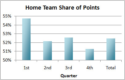
Below is the breakdown by quarter of the home team's share of points.



Overall, home teams score 52.5% of all points through the entire game. By far the largest advantage is seen in the 1st quarter, when home teams score 54.7% of the points scored during that period. The 2nd and 3rd quarters see a significant drop off, followed by the 4th quarter which shows the smallest advantage.

So just like the NBA, HFA in the NFL is primarily realized in the 1st quarter. Now let's compare how home teams fare when behind or ahead.



When trailing, home teams show the same pattern as the overall share in the 1st graph. But when ahead, home teams show no pattern, scoring about 59% of the points in each quarter. So there is a difference in the HFA effect not only by quarter, but by score difference as well.

Note that although trailing home teams score fewer than half of all points, this is what we'd expect. A team that's behind is likely the weaker team, so we would not necessarily expect them to outscore opponents, whether at home or not. This would not mean there is a home field disadvantage.

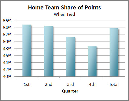
With that in mind, we can just look at points scored when the game is tied to (partially, at least) account for bias due to team strength.


Again, we see HFA diminish through the game. In fact, home teams score only 49% of points in the 4th quarter. My guess is that home teams that are tied in the fourth quarter have enjoyed 3 quarters of HFA, so they would tend to be the slightly weaker team without HFA. And since HFA becomes weakest in the 4th quarter, we're still seeing some bias due to team strength. In other words, it's better to be good than to be at home, especially in the 4th quarter.

This is more than just random trivia. Understanding how strong HFA is throughout the game helps us understand where HFA comes from. For example, as Marshall points out in his paper, it was commonly thought that HFA comes mostly from the crowd. It was expected therefore, that HFA would be strongest in the 4th quarter when crowds are typically loudest and most involved in the game, especially when the score is close. Also, if travel fatigue is the cause, then we'd expect HFA to be strongest toward the end of the game when fatigue becomes most important. But we see that the opposite is the case, so HFA may come from somewhere else.

I think there are probably multiple processes involved. There could be game-long effects, such as the crowd, but then there could be another process that diminishes as the game progresses. But whatever the underlying causes, HFA is strongest at the beginning of the game and diminishes as the clock winds down.

NFL Home Field Advantage and Team Strength

In my recent post about NBA and NFL home advantage I made the contention that the importance of home field advantage (HFA) increases when opponents are more evenly matched. I said this based on the results of this study, which looked at the importance of various factors in the playoffs. Because playoff games are relatively rare and offer a small sample size, I decided to look at regular season games that featured two playoff-caliber opponents in order to expand the data set. I noticed that home field advantage appeared stronger in games that featured "good vs good" teams or "bad vs. bad" teams compared to games that featured "good vs bad" match-ups.

Some commenters were understandably skeptical, so I dug a little deeper. I looked at all NFL regular season games from the 2002 through 2006 seasons (a total of 1280 games) and it turns out the effect appears real but not extremely consistent.

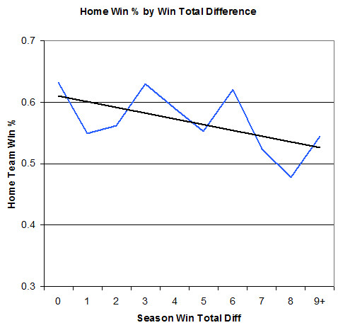
The graph below plots home team win percentage against season win total difference. For example, if a game featured a team that would eventually go 12-4 against a team that would end up 8-8, the season win total difference would be 4. As the gap between the relative strength of the opponents increases, HFA shrinks. For teams that end up with the same record, the home field advantage is relatively strong at 63% compared to an overall average of 57%.


Admittedly, the effect is not consistently smooth, which suggests there is a good deal of randomness involved. But the trend is fairly clear and it is consistent with what we observe in playoff games, not only in the NFL but the NBA as well.

On the other hand, if we accept the smoothed line, HFA ranges from 61% for evenly matched games down to 53% for mismatches. On the surface 8% doesn't seem very strong, but think of it this way: the effect of HFA ranges from +11% to +3%, a several-fold difference.

Bias and Home Advantage in the NBA vs. NFL

Recent attention has been focused on possible referee bias in the NBA. Former official Tim Donaghy, who is due to be sentenced for crimes related to fixing games, made allegations that officiating bias is common. The most damning accusation is that the NBA attempts to prolong playoff series by calling fouls more heavily on the team that is “up” in the series.

An article by Kevin Hasset, an economist and policy analyst for the American Enterprise Institute, points to apparent irregularities which he says could be evidence for NBA bias. Exhibit A is a large increase in home court advantage (HCA) from the regular season (60%) to the playoffs (74%). Exhibit B is the large discrepancy in fouls called against visiting teams compared to home teams. The author also points to suspicious examples where the difference in fouls and shooting percentage served to extend playoff series.

These results, however, are exactly what we should expect in a fair system. The explanation is due to how HCA affects different match-ups and the true cause and effect relationship between fouling and winning.

Home Field Advantage in the NFL

In the NFL, home field advantage (HFA) also increases from the regular season to the playoffs even though the league’s single-game playoff format provides no incentive to prolong a series. One big reason for the difference is due to the relative strength of opponents.

The NFL’s regular season HFA is 57%--the home team wins 57 out of 100 times. But in the playoffs it’s 68%. The biggest difference between regular season games and playoff games is the relative strength of opponents. Regular season games can feature mismatches, but playoff games feature only opponents who are relatively close in ability.

When teams are well-matched in ability, other factors such as HFA, which are normally small, appear more decisive. There are fewer cases of games that feature a strong visitor against a weak home team in the playoffs. The winning percentage of the home team would therefore naturally increase.

Home Court Advantage in the NBA

In the NBA, HCA is even stronger than the NFL’s HFA. Think of home advantage not as a game-long effect, but as a tiny advantage on each possession. The NBA plays quickly with a short shot clock and long 48 minute games. It’s a sport on speed. Each team gets about 100 possessions per game. Over the course of each possession, a HCA effect accrues into a very large game-long effect. HCA in the NBA is unusually strong for natural reasons having nothing to do with bias.

In the NBA playoffs, HCA is magnified by the same process at work in the NFL. Teams are closer in ability, and therefore other factors such as HCA appear to be more decisive.

Foul Calls and Home Court Advantage

Observers suspicious of NBA bias point to the fact that home teams are called for far fewer fouls than visiting teams. The correlation between numbers of called fouls and winning for the home team is quite clear. The natural conclusion would be that referees call more fouls on visitors --> therefore home teams tend to win. But I don’t think the direction of causation is clear at all.

If HCA is natural and not due to officiating bias, we’d still see the same results. Teams that are behind foul frequently toward the ends of games as a strategy. Losing teams know their best chance to win is to prevent their opponents from dribbling out the clock, and hope they miss a large number of free throws. In this respect, losing leads to fouling as least as much as fouling leads to losing. Even if referees were completely fair, we’d still see a disproportionate number of fouls called on visiting teams because visiting teams tend to be behind. The fouling effect would appear especially strong in the playoffs because HCA is especially strong.

This effect would also distort other stats such as shooting percentage. Teams that are behind would wisely take greater risks including taking more 3-point shots and playing a faster tempo. Over the long run this will depress their shooting percentage, but it’s the right strategy for the situation at hand.

Extending Series

Due to the format of the NBA’s 7-game playoff series, HCA will cause the illusion that referees are favoring the extension of a series. The NBA has changed its playoff formats slightly in recent years, but each format would roughly have the same effect. Currently, playoff series alternate home court this way: HH AA H A H. The finals are slightly different. That series goes: HH AAA HH. For every finals series however, there are 14 “regular” playoff series, so that format would dominate any study.

The 2-2-1-1-1 format would naturally give the appearance of favoring the extension of the series, even if referees were completely fair. Given that HCA is strong (74%) and normal (not due to bias), the most likely scenario is to have a 2-2 tie after game 4. In this case, the 5th game would probably be won by the home team. Game 6 goes to the home court of the team trailing 2-3 who will probably win. This extends the game to game 7.

The next two most likely scenarios are a 3-1 advantage going into game 5. Sometimes game 5 will be at the 3-win team’s home court, and sometimes it will be at the 1-win team’s home court. Given the 74% playoff win rate of the home team, at least half of these scenarios would therefore give the appearance of extending the series. (I say at least half because 3-1 advantages tend to go to stronger teams, which tend to start a series with home court.) So out of the 3 most likely scenarios, 2 tend to give the appearance of extending a series. The third “non-extending” situation is actually the least likely of the three. The only remaining scenario, the 4-0 sweep, is very rare.

Further, games in which the home team wins (and extends a series) would also naturally have more fouls called on the loser. This makes NBA officiating look all that more suspicious.

Whatever the reason, home advantage is real in all sports. It exists even when there are no incentives for a league to prolong competition, such as NCAA basketball or other pro sports. Basketball is particularly susceptible to accusations of bias at all levels due to its high frequency and subjectivity of foul calling. Referee judgment is heavily involved in determining outcomes. To be honest, I wouldn’t be surprised if the NBA did somehow tilt things in the interest of better TV ratings. But the evidence needs to be completely understood before we can make any conclusions.

A follow up on the NFL's HFA and team strength here.

Phil Birnbaum's take here.

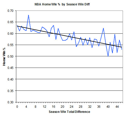
Addendum: Here is a plot of NBA regular season home team win percentage according to the difference in opponent season wins.

As the difference in team strength increases HCA decreases. However, even at a difference of zero wins, HCA tops out at 64%, short of the 72% in the playoffs over the past two seasons. But over the span of 1996 through 2007, the HCA in the playoffs was 67%. So there may be something special about the playoffs that increases HCA. Sold-out arenas, national attention, and intensity might explain the difference. There may be one more reason too. The stronger (higher seeded) teams get more home games in the playoffs due to the 2-2-1-1-1 format, so there could be some significant covariance between relative team strength and HCA.

Cold Weather Effect on Scoring

In a recent post I theorized that the sudden importance of run defense in the playoffs might be due to cold weather. This post will continue that line of analysis and look at the effect of cold weather on scoring.

The past weekend's conference championship games were played in frigid weather. It seemed that expert after expert remarked that cold weather would keep the scoring down. Certainly it makes sense to anyone who's played sports in extremely cold weather. It definitely makes it harder to throw, catch, and even kick. But it's just as cold for defenses as for offenses. So does cold weather really keep NFL scores lower?

Here are the average home and visitor scores for various circumstances. The first column is for all regular season games in the 2002-2006 seasons (n=1280), and the second column is for those games played in cold climates (n=114), as defined here. Since many playoff games are played in cold weather, the third column is for all playoff games (n=50+5). (Super Bowl scores are not included because there is no home advantage.)

	Reg. Season	Cold	Playoff
Home	22.3	22.5	25.0
Visitor	19.8	18.6	19.9

The second table looks at scores from the same sets of games differently. The average scores of the winning and losing teams are listed. (Super Bowl scores are included as playoff games here.)

	Reg. Season	Cold	Playoff
Winner	26.8	27.0	28.9
Loser	15.3	14.1	16.5

Cold weather doesn't appear to have a large effect on scoring. It seems to slightly enhance the spread between winner and loser by depressing the score of the loser. This is likely due to the "dome at cold" effect discussed in previous posts.

Playoff scores are generally higher, both in terms of winner and loser, and for the home and visiting teams.

It doesn't appear that cold weather reduces scoring.

I can understand where the perception might come from. Because dome teams are at a disadvantage playing outdoors in cold weather, it follows that they would score less. Many competitive dome teams in recent years have been ones with fast-scoring offenses. The Vikings, Rams, and Colts of recent memories all featured very strong offenses. When these teams were competitive late in the season (and when people were paying attention to them), they would be expected to score less when playing outdoors. But this effect on dome teams would be limited to these specific circumstances and not affect teams in general.

When the Giants played in Green Bay or the Chargers played in Foxboro yesterday, we should not have expected low scores due to the cold temps. Although the frigid sub-zero temperatures yesterday were extreme, even for Green Bay standards, the point is that the weather affects both offense and defense.

Road Winners in the Playoffs

One notable difference between the regular season and the playoffs is that the higher seeded playoff team hosts the game. If the seedings reflect the actual strength of the teams, we should expect to see a larger winning percentage for home teams than in the regular season. Teams that win on the road through the playoffs would be truly remarkable teams.

In this post I'll look at road winners in each round of the playoffs from 1994, the year the salary cap began, through 2006, the most recent year. I'll also look at differences in road winners from two different playoff periods. The first period is from 1994-2001, when the playoffs featured 3 division winners and 1 wildcard team from each conference. The second period is from 2002-2006 when the playoffs featured a 4th division winner and two wildcard teams. The sample sizes aren't terribly large, but large enough to begin to see some possible trends.

The first table lists each round of the playoffs for the entire post-salary cap period, and the number and percentage of road winners. Overall road teams won 33% of games in the playoffs. This is in contrast to the normal 42-43% rate in the regular season.

1994-2006	Games	Road Wins	Road Win%
Conference	26	11	42
Division	52	13	25
Wildcard	52	15	29
All Rounds	130	39	32

The next two tables break up the data into the two playoff periods. The first table lists the road winners from '94-'01. The second table lists them from '02-'06, featuring the NFL's current playoff structure.

1994-2001	Games	Road Wins	Road Win%
Conference	16	6	38
Division	32	7	22
Wildcard	32	7	22
All Rounds	75	20	29

2002-2006	Games	Road Wins	Road Win%
Conference	10	5	50
Division	20	6	30
Wildcard	20	8	40
All Rounds	50	19	40

Again, the sample sizes aren't large, but we can make some observations. First, the playoff seedings do appear to reflect a stronger home team winning percentage. The better team is probably seeded higher and hosts the game. But this effect could also be due to the "dome at cold" effect. With bitter cold weather in most cities in January, dome teams would be at a severe disadvantage when playing on the road outdoors. In fact, of the 14 "dome at cold" match-ups, dome teams have won only 2 (14%), which is same the rate as in December in the regular season.

The conference championship games reflect a relatively high number of road winners (40%). This makes sense for a couple reasons. Low-seeded dome teams have already been eliminated. Also, the games feature the closest match-up between relative team strength. They ostensibly would feature the two best teams at the time (the true 1 and 2 seeds), regardless of their official seeding.

Third, there is a noticeable difference between the '94-'01 wildcard rounds and those of '02-'06. Road teams have been winning more frequently lately in the wildcard round (40%, vs 29%). There isn't enough data yet to make any firm conclusions, but it makes sense intuitively.

I think we're seeing more road winners or "seed"-upsets due to the new division structure. With four division winners in each conference, it's more likely an average team can luck into the division championship, especially with a weak division. With only four teams in each (compared to five or six previously), it's more likely to have a thoroughly weak division. The wildcard teams, which are road teams by rule, are probably from the stronger divisions and possibly stronger teams than their seeding indicates. Similar to the conference championship games, the modern wildcard round feature games between closely seeded teams (5 vs. 4) and (3 vs. 6).

This year, the two 5 vs. 4 seed games are expected to be toss-ups. JAX is slightly favored over division-winner PIT by 2.5 points, and TB is favored over NYG by 2.5 points. SEA, the division winner of the clearly weakest division, is only favored over WAS by 3.5 points.

'Dome at Cold'

This week features two of the three "dome team at cold weather" games of the 2007 season. Earlier, CIN defeated STL in week 14. Today CHI hosts NO and GB hosts DET.

Dome teams are at a severe disadvantage when playing in cold weather. Over the past five regular seasons, they've won only about 14% of the time in those situations. Accounting for relative team strength, they would be expected to win only 12% of the time.

GB is already a heavy favorite over DET, and the weather factor would only enhance GB's expected chance of winning. But the game prediction model features closer odds for the NO at CHI game. NO is favored with a 0.57 probability of winning.

However, when the weather is factored in CHI is going to be favored. Replacing the standard home field advantage coefficient with the "dome at cold" coefficient we get a 0.62 win probability for CHI.

With the weather factor, GB becomes a heavier favorite at 0.92.

Some people are already looking ahead to the likely AFC championship match-up between IND and NE. Although IND played NE very well, and nearly won the game earlier in the year without five starters, their next game will be very different. It will be in Foxboro, Mass. in late January. It was no fluke that the one year IND was able to get past NE to get to the Super Bowl was the year they hosted the game.

Winning on the Road

Teams with good running offenses do not win any more road games than other teams, all things being equal. That's right--being good at running the ball does not help teams win on the road. Contrary to what we've been told for years, having strong passing game is far more important to visiting teams than having a good running game.

Let me make a clarification up front. I'm not suggesting that having a great running performance in an individual road game doesn't help win that game. I'm saying that being a "running team" doesn't help win on the road. Teams that are "built" to win on the road are those that pass well and don't fumble.

I stumbled on this somewhat by accident when I was studying the effect of climate on home field advantage. My usual game model is a logistic regression that estimates the probability of winning based on team efficiency stats and home field. A simplified version looks like this:

Team A season efficiency stats
Team B season efficiency stats
Team A at home [1 if true, 0 if false]

This method resulted in balanced weights for the coefficients for Team A and Team B, and the importance of home field was captured in the coefficient for 'Team A at home.' But during my research into climate effects, I decided to try an alternate model without the home field variable. It looked like this:

Visiting team season efficiency stats
Home team season efficiency stats

With this method we would expect unbalanced coefficients. Because home teams win more often, the coefficients for the home team were generally stronger than for the visiting team. This means that if two theoretically equal teams played, the home team would have a higher probability of winning, which is exactly what we observe.

By examining the imbalance of each stat we can see what kind of teams tend to win on the road. Here are the regression coefficients for each efficiency stat for both home and visiting teams. (Logisitic regression is more difficult to interpret than linear regression. The coefficients indicate the change in the log of the odds ratio of the outcome. But we are comparing the relative strength of each coefficient, so don't worry about the "log odds ratio" for now. Just pay attention to the relative size of the coefficient between home and away team stats.)

Team Stat	Home Coeff	Visitor Coeff
O Pass	0.40	-0.49
O Run	0.48	-0.04*
D Pass	-0.60	0.48
D Run	-0.27	0.16
O Int Rate	-16.40	15.61
D Int Rate	19.30	-17.63
O Fum Rate	-11.57	30.77
Pen Rate	-1.65	1.30

The model has very solid goodness-of-fit stats, and it is 69.9% accurate (retrodictively) in predicting game winners. The regression is based on all regular season game outcomes in the past five years (n=1280).

First, compare the coefficients for offensive passing efficiency. The coefficient for home teams is 0.40, and for visiting teams is 0.49. We can interpret these numbers by saying "having a good passing game is slightly more important in winning for the visiting team than for the home team." But the difference is slight, and may not be significant.

Next, compare the coefficients for offensive running efficiency. The coefficient for home teams is 0.48, but for visiting teams it is only 0.04--practically zero! (The difference of 0.44 is strongly significant.) The near-zero coefficient for visiting teams' offensive running efficiency is what tells us that running well simply doesn't matter on the road.

Also, for some reason, teams that tend to fumble more often than others are at a greater disadvantage as visiting teams. And conversely, teams that don't fumble tend to have a greater advantage as road teams.

There are imbalances between nearly all of the team efficiency stats, but none as stark as that for offensive running. This was such an unexpected result and I had no prior theoretical basis for the observation, so I confirmed the results with a simpler analysis using correlation coefficients.

For each team over the past 5 seasons (n=160), I added up their road and home wins. The correlations of each efficiency stat with home and road wins were calculated. If different stats affect a team's ability to win at home and on the road differently, as we saw in the regression, then we should see different correlation coefficients. For example, the correlation between offensive running efficiency and home wins should be much stronger than running and road wins.

	O Pass	O Run	O Int Rate	O Fum Rate	D Pass	D Run	D Int Rate	Pen Rate
Away Wins	0.55	0.10	-0.40	-0.42	-0.34	0.00	0.31	-0.16
Home Wins	0.48	0.22	-0.36	-0.36	-0.45	-0.07	0.36	-0.17

The correlations confirm the results from the regression. Being a good running team is more important to winning when at home, and not nearly as important to the visiting team. (Also note that stopping the run is just not important whether on the road or at home, as we've seen in previous research.)

I also did an even simpler analysis by comparing the average season running efficiency stats of all road winners and for all home winners. Again, the data was from every regular season game over the past five years (n=1280). The average offensive running efficiency for road winners was 4.13 yds/rush and for road losers was 4.10 yds/rush--a difference of only 0.03 yds/rush.

We see the opposite with passing efficiency. Road winners average 6.18 yds/att and road losers average 5.90 yds/att--a difference of 0.28 yds/att which is about 9 times larger than the difference we found for running. Again we see indications that passing efficiency tends to be the more important stat for the road team.

The obvious question is "why?" Why doesn't being a capable running team help win road games? My only theory is that passing well helps come from behind far more than running well. If road teams tend to find themselves behind more often than home teams, then unless they can pass, they wouldn't be able to score quickly and come back from a deficit. But home teams need to come back from deficits too, so the reason why running teams don't win on the road remains puzzling.

NFL Home Field Advantage by Climate 2

In a previous post, I looked at how home field advantage is affected by weather. Each NFL city was categorized by its December climate--dome, warm, moderate, and cold. By comparing the winning percentage of home teams in games in the early season (weeks 1-12) and the late season (13-17) the effect of cold weather was estimated.

In this post, the effect of cold weather on home field advantage will be measured more precisely. By using logistic regression, relative team strength is accounted for. In addition, the statistical significance of the observed weather effect indicates if the effect is real and systematic, or just a result of luck and small sample size.

The last post left off with this table. The left most column describes the visiting team's climate, and the top row describes the home team's climate. For each combination of visiting and home climate, the change in home team winning percentage from early to late in the season is listed. Positive numbers indicate that cold weather may favor the home team. For example, when dome teams play at warm cities, the home team winning percentage was 20% higher late in the season than early in the season. But when dome teams play at moderate cities, the home team winning percentage appeared to be 9% lower late in the season.

Difference	Dome	Warm	Mod	Cold
Dome	0%	+20	-9	+35
Warm	-5	+14	-7	-3
Mod	-8	-24	-6	-13
Cold	-8	+2	-15	+8

Several match-ups indicate that the cold and wind of late-season outdoor football has an effect on HFA. Consistent with other research, it appears that dome teams suffer when playing in cold climates.

Another remarkable combination is moderate weather teams playing in warm cities (-24%). But it's not clear why moderate teams would have an easier time playing in the balmy breezes of Florida or San Diego in December. Other notable match-ups are dome teams playing at warm cities (+20%), and cold teams playing at moderate cities (-15%).

To determine if the observed differences in HFA between early and late season games is really due to the change of weather, and not due to relative team strength or luck, several logistic regression models were run. The models were based on every regular season game from the 2002 through 2006 seasons (n=1280). For each game, each team was designated either Team A or Team B. The general model specification was the following:

Dependent variable:
Team A won

Independent variables:
Team A season efficiency stats
Team B season efficiency stats
AHome
[Weather dummy variable]

The team efficiency stats include offensive and defensive passing and running efficiency, turnover rates, and penalty rates. AHome is a dummy variable that is 0 when Team A is away and 1 when Team A is home. The [Weather dummy variable] is 1 when the particular climate match-up of interest is present for the game, and 0 when otherwise.

A general HFA variable (AHome) was included to isolate the effect of weather from the general home field advantage due to travel, psychology, officiating, or other effects.

Several models were run for each climate match-up of interest. The table below lists the statistical significance of the 'weather variable' and the resulting home field advantage calculated from the regression results. Note that the overall HFA rate is 57.5%.

Visitor	Home	p-value	HFA (%)
Dome	Cold	0.03*	88
Dome	Warm	0.28	75
Warm	Warm	0.58	71
Warm	Cold	0.74	76
Mod	Warm	0.11	40
Mod	Cold	0.95	62
Cold	Mod	0.13	49

Accounting for relative team strength, the only truly significant result is for dome teams in cold weather (p=0.03), with an expected home team winning percentage of 88%. This result is confirmed by the actual 86% home team winning percentage when dome teams play at cold cities late in the year. The regression's estimate of 88% suggests that the cold city home teams may have been slightly weaker compared to their dome opponents over the past 5 years.

Two other types of match-ups might be considered marginally significant--moderate teams at warm cities (p=0.11), and cold teams at moderate cities (p=0.13). Both results indicate a reduced HFA later in the season for those match-up types. But since there were 16 combinations of climate match-ups, chances were that we could see one or two type-I errors, i.e. see significance when none is truly there. Because there is no a priori theoretical reason why to expect those results, we shouldn't deem them significant.

Finally, one last model specification was run to make sure no other climate match-up types were significant. The final model included all late-season match-ups types together. No additional types were significant.

It's clear that the situation of a dome team playing playing in a cold city late in the season creates a much stronger HFA than normal. But a larger data set is needed to conclusively analyze other weather match-ups. Dividing 1280 games into 16 types of match-ups and 2 weather periods creates small sub-samples.

A prediction model's accuracy may benefit from enhancing the weight of HFA in certain situations. Looking ahead, there are only three 'dome at cold' match-ups in 2007. STL travels to CIN in week 14, and NO visits CHI and DET visits GB in week 17.

NFL Home Field Advantage by Climate

In this post I'll begin an analysis of home field advantage in the NFL and its relationship to climate. Others have examined the connection between weather and HFA previously, but here I'll attempt to present the data with a clear and novel approach. This post represents the 'clear' part. In following posts, the novel part will use logistic regression to account for team strength and determine the significance of each particular type of climate match-up.

I began by dividing each home city into four categories: dome, cold, moderate, and warm based on a combination of each city's average December high temperature and wind speed. The dome cities include STL, NO, MIN, DET, IND, and ATL. The cold cities are GB, BUF, CLE, CHI, KC, DEN, NYG, NYJ, NE, PHI, PIT, and CIN. Moderate cities include BAL, WAS, CAR, SEA, OAK, SF, TEN, and DAL. The warm cities are MIA, TB, JAX, HOU, SD, and ARI.

Based on all NFL regular season games from the 2002 through 2006 seasons, the winning percentage of the home team was calculated for each type of climate match-up. I divided the season into "early" and "late." The early season is defined as weeks 1 through 12 and the late season is defined as weeks 13 through 17. For example, the winning percentage of the home team in match-ups of cold teams at moderate cities in the early season is 57%, with n=77 examples of such cases.

The home winning percentage of all types of weather match-ups are presented below in a series of pairs of tables. Each table is presented the same way, with the visiting team climate on the left and the home climate on the top. The first table in each pair is for the early season (pre-December), and the second table is for the late season (December games).

Sample size is usually an issue when populations are divided up among several classes. For that reason, the first pair of tables lists the number of cases of each type. For example, the top right cell of the first table lists the number of games featuring dome teams playing at cold cities in the early season. The same cell in the second table lists the same type of match-up in the late season.

Wk 1-12	Dome	Warm	Mod	Cold
Dome	31	29	44	62
Warm	34	20	50	62
Mod	40	49	51	78
Cold	59	66	77	128

Wk 13-17	Dome	Warm	Mod	Cold
Dome	15	17	21	21
Warm	16	11	17	30
Mod	25	20	17	40
Cold	20	28	43	59

The second pair of tables simply lists the straight-up winning percentage of the home team in each type of match-up. For example, the bottom left cell of the first table lists the home team winning percentage when cold teams play at domes in the early season. The same cell in the second table lists home winning percentage of cold teams at domes in the late season.

Wk 1-12	Dome	Warm	Mod	Cold
Dome	61%	45	61	51
Warm	68	50	66	66
Mod	60	59	59	76
Cold	53	52	57	50

Wk 13-17	Dome	Warm	Mod	Cold
Dome	61%	65	52	86
Warm	63	64	59	63
Mod	52	35	53	63
Cold	45	54	42	58

What immediately stands out is the very high winning percentage of cold teams hosting dome teams late in the season. The most remarkable result, however, may be the 35% home winning percentage of warm teams hosting moderate teams. Note that there are only about 20 cases of each type of match-up in the past 5 years, so these results could be due to luck or due to general team strengths of the according type of teams. Perhaps a couple moderate teams have been relatively dominant over warm weather division rivals between '02 and '06.

The final table lists the difference in home winning percentage between late season and early season match-ups. Simply put, it is late season winning percentage minus early season winning percentage. A high positive number indicates cold weather may give an advantage to the home team. A negative number or near-zero number suggests otherwise. We'd expect to see a zero for dome teams at dome teams, because outdoor weather is obviously not a factor. This method begins to account for relative team strengths over the period studied.

Difference	Dome	Warm	Mod	Cold
Dome	0%	20	-9	35
Warm	-5	14	-7	-3
Mod	-8	-24	-6	-13
Cold	-8	2	-15	8

Take dome teams for example. By reading across, we see that dome teams seem to have no greater HFA in late season than the early season against other dome teams--as we'd expect. We also see that they are at a 20% disadvantage playing at warm cities but, for some reason, have a 9% better advantage playing at moderate cities late rather than early. Lastly, we see that dome teams appear to be at a severe disadvantage playing in cold cities late in the season, apparently giving up 35% advantage to the cold.

As mentioned above, some of the observed differences in HFA due to weather may be due to luck and relative team strengths among the weather-classes. The final table is a simple way of accounting for team strength, but it does not address the possibility that the differences are primarily due to luck. The final part of this article will use logistic regression to more powerfully account for team strength and test for statistical significance.

Weather and Home Field Advantage

Someone recently pointed out a study that indicated home field advantage (HFA) is not the same for every stadium. While that's certainly true, it's very hard to quantify. By definition, the same team is always the home team when measuring a particular location's HFA, so in any given year there would be a lot of team strength captured in a variable accounting for the field's HFA.

The efficiency model I've used includes a factor for HFA, but it is the same regardless of climate. This is the beginning of an effort to quantify the effect of climate on HFA and to see how much of HFA is due to climate differences and how much is due to other factors such as crowd noise, referee psychology, or travel.

The table below lists each home team along with their average December weather. Click on the table headers to sort

Team	Avg Dec T	Avg Dec Wind	Wind Chill
GB	29	10.5	19.7
BUF	36	13.3	27.3
CLE	37	12.1	29.0
CHI	37	11.0	29.5
NE	42	12.2	35.3
KC	42	11.2	35.7
PIT	42	10.4	36.0
NYG	44	10.8	38.3
NYJ	44	10.8	38.3
CIN	44	10.2	38.5
PHI	44	10.1	38.6
DEN	44	8.4	39.3
SEA	46	9.5	41.3
WAS	46	7.8	42.0
BAL	49	9.3	45.0
TEN	49	8.9	45.2
CAR	54	7.4	51.9
SF	56	7.1	54.4
DAL	57	10.8	54.5
OAK	58	7.1	56.8
HOU	65	8.0	65.0
ARI	65	5.1	65.8
JAX	66	7.8	66.3
SD	66	5.6	66.8
TB	72	8.4	73.5
MIA	75	9.2	77.1
ATL	70	0.0	79.2
DET	70	0.0	79.2
IND	70	0.0	79.2
MIN	70	0.0	79.2
NO	70	0.0	79.2
STL	70	0.0	79.2

It's not a surprise that Green Bay is coldest by far, followed by places such as Buffalo, Cleveland, and Chicago. Green Bay would even qualify as a cold climate through November with an average 36 deg wind chill. But I was surprised by how much colder (and windier) a place like Kansas City is than Baltimore or Washington. I'm still considering how to classify each city. Domes are easy, but where is the line drawn between cold and moderate? Should there be cold, moderate, and "warm" classes? For now I'd put the line between cold and moderate at 40 deg wind chill, between DEN and SEA. I'd also define warm weather teams starting at 60 deg between OAK and HOU.

Continue reading this article here.