Bayesian Draft Prediction Model

Let's say you're a GM in need of a safety. You really like Ha Ha Clinton-Dix (FS Ala.) but are unsure if he'll still be on the board when you're on the clock. Do you need to trade up? How far? What if you're a GM with a high pick and would be willing to trade down if you're still assured of getting Clinton-Dix? How far down could you trade and still get your guy?

I've created a tool for predicting when players will come off the board. This isn't a simple average of projections. Instead, it's a complete model based on the concept of Bayesian inference. Bayesian models have an uncanny knack for accurate projections if done properly. I won't go into the details of how Bayesian inference works in this post and save that for another article. This post is intended to illustrate the potential of this decision support tool.

Bayesian models begin with a 'prior' probability distribution, used as a reasonable first guess. Then that guess is refined as we add new information. It works the same way your brain does (hopefully). As more information is added, your prior belief is either confirmed or revised to some degree. The degree to which it is refined is a function of how reliable the new information is. This draft projection model works the same way.

For a prior estimate of when each prospect might be taken, I created a probability distribution centered around a consensus of best-player rankings. Some guys call them the big-board rankings. I used sources including Scouts, Inc. top 150, CBS Sports top 300, Kiper's top 100, Gil Brandt's top 125. (In this case, a probability distribution is an assignment of a probability that a prospect of interest will be taken at each pick in the draft. A simple example might be Jadeveon Clowney's distribution, which would be something like 90% for pick #1, 8% for pick #2, and 2% for the next few picks. In other words, it's highly likely he goes at or near the top of the draft.)

The key at this stage is that this prior distribution is only as confident as these types of projections have been in the past. The distribution is based on the errors of these rankings over the past four years. They don't take into account team needs or when certain teams have picks, so we shouldn't expect the accuracy to be great. But that's ok, because for now we just need a reasonable first guess. The chart below depicts Clinton-nix's probabilities of selection at each pick in the draft based solely on best-player rankings.

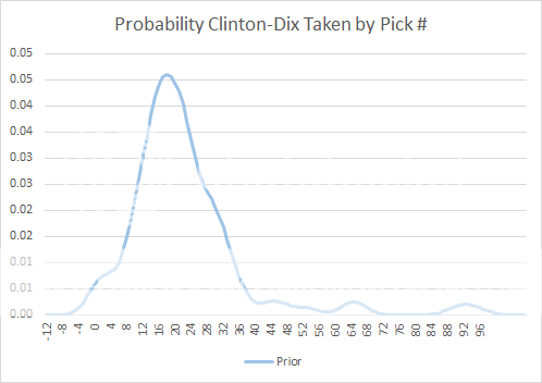
The chart above illustrates our a priori belief about when he could be taken. This is based on his overall big- board ranking, together with a function of how accurate those rankings have been. Clinton-Dix's consensus ranking is 19th, so we see that his distribution is centered around the 19th pick as we'd expect. You might have noticed there is some positive probability that he would be selected before the draft even begins with the -4th pick. Don't worry--that will work itself out.

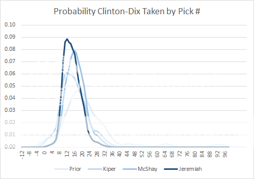
Using Bayesian inference, let's add expert draft projections, which do account for team needs and draft order, starting with Mel Kiper's projection. He (Kiper, not Bayes) predicts Clinton-Dix will go at #10. In the chart below, The next darker shade of blue is our estimate after adding Kiper's projection. Keep in mind that the weight of each addition of new information is only as strong as the information has proved to be accurate in the past.

 The next darker shade in the next chart is the resulting estimate after we add Todd McShay's projection. He also says Clinton-Dix will go at #10. As you can see, the probability distribution is getting narrower (more precise) and is inching closer to 10.

Next I added Daniel Jeremiah's (NFL Network) projection to the mix, and he has Clinton-Dix going at 13. The probabilities are now converging and becoming even more precise, which is to say more confident. The more expert input we add, the better the prediction. The chart really captures how Bayesian inference works to refine projections with new information.

The model projects Clinton-Dix is most likely to be taken with pick 12 or 13, but there's only about a 9% chance that he'll be taken exactly at 12. There's still a lot of uncertainty, and that's to be expected. If you look at the historical accuracy of draft projections, there are always unexpected twists and surprises. Don't kid yourself. There is almost no way to predict exactly when each player will be taken, especially after the 1st few picks. The very best 'mocks' only get 11 or 12 of the 1st round picks correct in any given draft.

The good news is that we don't have to be so concerned about exactly which pick is used for a player. From the point of view of a GM, it's valuable to simply know whether a player will still be available at a given pick number, which is a slightly easier question to answer.

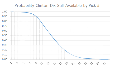
The last chart takes the final result and turns it into what's called a cumulative probability distribution. It shows the probabilities that Clinton-Dix will still be available at each round of the draft. This could be immensely useful to a team, (especially for picks that aren't so obvious). For example, if a team really coveted Clinton-Dix, they'd have to trade up to pick 9 for a 90% confidence level he'll still be on the board, and to pick 8 for a 95% confidence level. Also, if a team wanted him and had a very high pick, they could trade down as low as 9 and still feel 90% sure they'd get him.

Even if a trade isn't in the cards, this approach might still be useful. Say a team needs both an OT and a S, and the GM is considering one player at each position for his 1st round pick. And say the model shows there is another top tier safety probably still available at his team's 2nd round pick, but all the top tier OTs would probably be off the board. That should tilt the balance toward taking the OT in the 1st and the S in the 2nd.

The beauty of this approach is its flexibility. We could add any amount of information to improve the estimates. If you don't care for Mel or McShay, we can easily replace their projections with any other set, including those of a team. We could add a team-need input or whether a player visited a particular team. There is lots of room for enhancements.

As the draft is conducted, these estimates can be updated in real-time. As each selection is made, the probabilities for the remaining players can be adjusted simply by assigning a zero probability to the recent pick #, and then recalibrating the rest of their probabilities.

I'll go over more details and the math behind the model in another post. I'll also publish an interactive tool (sneak peek above) to see every prospect's probabilities. Stay tuned for more. But for now, here are the key points regarding this model:

1. The draft is a lot less predictable than people make it out to be.
2. Aggregating expert projections will tend to be more accurate than a single projection, as long as the aggregation is done right.
3. The prior distribution doesn't need to be perfect, just a reasonable starting point.
4. The inputs to the model are weighted only as much as they have proven to be accurate in the past.
5. The final result has all the uncertainty of the system baked in.
6. We don't always need to know exactly when a player will be chosen. Often it's very useful to know whether or not he's still available at a certain pick.