The new Bayesian draft model is nearly ready for prime time. Before I launch the full tool publicly, I need to finish describing how it works. Previously, I described its purpose and general approach. And my most recent post described the theoretical underpinnings of Bayesian inference as applied to draft projections. This post will provide more detail on the model's empirical basis.
To review, the purpose of the model is to provide support for decisions. Teams considering trades need the best estimates possible about the likelihood of specific player availability at each pick number. Knowing player availability also plays an important role in deciding which positions to focus on in each round. Plus, it's fun for fans who follow the draft to see which prospects will likely be available to their teams. Hopefully, this tool sits at the intersection of Things helpful to teams and Things interesting to fans.
Since I went over the math in the previous post, I'll dig right into how the probability distributions that comprise the 'priors' and 'likelihoods' were derived.
I collected three sets of data from the last four drafts--best player rankings, expert draft projections (mock drafts), and actual draft selections. In a nutshell, to produce the prior distribution, I compared how close each player's consensus 'best-player' ranking was to his actual selection. And to produce the likelihood distributions I compared how close each player's actual selection was to the experts' mock projections.
Consensus Best Player Rankings
The prior distribution only needs to get us in the ballpark, and be approximately of the right shape. In this model, the prior is based on a consensus of best player available rankings. Best player rankings are overall rankings without regard to exactly where they would fit in the draft based on things like position or team need. I averaged rankings from ESPN's top 300, CBS Sports top 300, Gil Brandt's top 125, Kiper's top 100, and Scouts Inc.'s top 150.
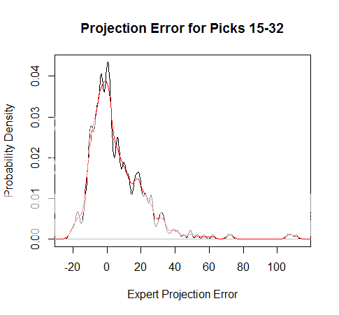
Over the past four years, the consensus rankings are very good starting points for predicting when a player will be taken, but are rarely spot-on accurate. I assessed the accuracy of the rankings as predictors by looking at the distribution of each selection's error. In other words, how often was the ranking spot-on? What proportion of the time was it off by 1 pick late? 1 pick early? 2 picks late? etc...
This produced the plot below. The black line is the observed proportion of each degree of error. (It should actually be a probability mass rather than a density because the picks are discrete numbers, not a continuous variable. But for the sake of clarity, I plotted the distributions as densities. The results are unchanged.) An error of -1 means the player was actually chosen 1 pick earlier than his overall rank. An error of +1 means the players was actually chosen 1 pick later than his overall rank, and so on.

It's much easier to predict the pick # of the very top prospects than the third-day prospects of the 4th round and later. Not only is there far more attention and analysis for the top players, but there is a bound to the error of any prediction--You can't have a player chosen before the 1st pick. Because accuracy is largely dependent on where players are generally ranked, I created separate distributions for different regions of the draft. The one depicted above happens to be from the second half of the 1st round. I divided the prospects into groups of 1-5, 6-14, 15-32, 2nd round, 3rd round, and later.
You might have noticed that if the 15th best ranked player has an error of -20, that would mean he was actually 5 picks before the draft began. That's a result of aggregating the players into groups. Ideally, I'd prefer unique distributions for every individual pick #, but that's impossible given the amount of data available. To correct for the "negative pick #" flaw, I reallocated any probability mass that fell before the #1 pick into the positive region, by setting the probability of being picked before #1 to zero, and adjusting the rest of the distribution so it summed to 1.
Expert Projections
The Bayesian 'likelihoods' were computed based on expert mock drafts using the same general techniques, with one important difference. As discussed in the previous post, Bayesian inference relies on inductive reasoning.
The prior distribution is the probability a player was taken with each selection number given his overall ranking. But the likelihood looks at the question from the other direction. The likelihood distribution is the probability a player was projected to be taken at each selection given when he was actually chosen. For instance, 'what's the probability the player who was actually chosen 10th was projected to be taken 10th? Projected to be taken 9th? 11th? Etc...
I treated each expert as a clone, using the assumption no one expert is significantly better than another, assuming the experts considered are among the most serious and most widely respected. While I would grant that one guy might be 'truly' better than another, it's probably very close, and we might need 100 years worth of data to tell with any degree of confidence. I'd prefer to have unique distributions for each expert, but that creates distributions that are too sparse. To establish the likelihood distributions, I used Kiper, McShay, and Mayock, but also included a couple additional mocks from Sports Illustrated and CBS Sports to round out the data.
Again, using the bkde function in R's Kern Smooth package, I created smoothed estimates of the likelihood distribution.
The complete results of the model applied to all of this year's prospects will be published soon.