Shameless Plug for Win Probability Site

Amaze your friends. Wow your family. Dazzle your co-workers. Confuse your brother-in-law.

Don't forget to fire up the Super Bowl XLIII in-game win probabilities this Sunday. Them: "Oh man, they'll never come back from that lead!" You: "Actually, they have a 15% chance of coming back" Them: "Shut up, you smart ass. Why do you have to suck the fun out of everything?"

Actually, that could be a pretty good catch line for my site. "Advanced NFL Stats: Sucking all the fun out of football since 2007!"

And as a bonus, for every click on the win probability site Sunday, a portion of the proceeds will go to the Get a Steeler Fan His G.E.D. Fund.

Super Bowl Winner Stats

Last year I looked at how often teams won playoff games based on their season-long performance in various categories. I basically looked at how predictive various stats are in forecasting playoff wins. For example, how often does the team with the better passing efficiency win? I learned some interesting things such as how important run defense appears to become in the playoffs.

This time around I looked at just Super Bowls. How often does the team with the better season-long performance in each category win the big game? The sample size is very small, but the Super Bowl is a unique game in many ways, so we might learn something.

I only looked at Super Bowls since Super Bowl XV, the 1980 game between the Raiders and Eagles. In 1978, the passing rules changed and significantly altered the sport, but the league did not adjust for another couple years. Yes, this shrinks the sample to just 28 games, but I’m not going for statistical conclusions, just an initial look to see if anything stands out. No fancy regressions this time, just straightforward percentages.

The results are in the table below. You can read it as saying “the team with the better [efficiency stat] won the Super Bowl [x%] of the time.”

Stat	Win %
O Pass	50
O Run	57
O Int	61
D Pass	61
D Run	46
D Int	54

I’m a little surprised that the team with the better offensive passing efficiency only won 50% of the time. I’d think that would be a fairly solid advantage. Defensive passing looks like it might be the more important category.

Also, defensive run efficiency doesn’t appear to hold the same importance that it has in the playoffs lately. The better run-stopping team only won 46% of the time.

But again, we can’t really draw any conclusions. There are only 28 games in the sample, so a single game swings the percentage by about 3%.

In case you’re curious, the Steelers have the advantage in offensive running and all the defensive categories. The Cardinals have the better offensive passing efficiency and the lower interception rate.

How the Model Works--A Detailed Example Part 2

This is a continuation of an article that details exactly how my predictions and rankings are derived. You can read part 1 here. To recap, I'm using the Super Bowl match-up between the Steelers and Cardinals as an example. So far, we've used a logistic regression model based on team efficiency stats to estimate the probability each team will win.

We haven't accounted for strength of schedule yet. For example, the Steelers may have the NFL's best run defense, yielding only 3.3 yds per rush. But is that because they're good or because their opponents happened to have poor running games?

To adjust for opponent strength, we'll first need to calculate each team’s generic win probability (GWP), or the probability of winning a game against a notional league-average opponent at a neutral site. This would give us a good estimate of a team’s expected winning percentage based on their stats.

Since we already know each team’s logit components, all we need to know is the NFL-average logit. If we take the average efficiency stats and apply the model coefficients we get Logit (Avg) = -2.52.

Therefore, for the Cardinals, a game against a notional average opponent would look like:

Logit = Logit (ARI) – Logit (Avg)
= 0.07

The odds ratio is e^0.07 = 1.09. Arizona’s GWP is 0.52—just barely above average. If we do the same thing for Pittsburgh, we get a GWP of 0.73. And it’s easy enough to do for all 32 teams. In fact, that’s what we need to do for our next step in the process, which is to adjust for average opponent strength.

The GWPs I calculated for Arizona and Pittsburgh were based on raw efficiency stats, unadjusted for opponent strength. That’s ok if we assume they had roughly the same strength of schedule. But often teams don’t, especially in the earlier weeks of the season.

To adjust for opponent strength, I could adjust each team efficiency stat according to the average opponents’ corresponding stat. In other words, I could adjust the Cardinals’ passing efficiency according to their opponents’ average defensive efficiency. I’d have to do that for all the stats in the model, which would be insanely complex. But I have a simpler method that produces the same results.

For each team, I average its to-date opponents’ GWP to measure strength of schedule. This season Arizona’s average opponent GWP was 0.51—essentially average. I can compute the average logit of Arizona’s opponents by reversing the process I’ve used so far.

The odds ratio for the Cardinals’ average opponent is 0.51/(1-0.51) = 1.03. The log of the odds ratio, or logit, is log(1.03) = 0.034. I can add that adjustment into the logit equation we used to get their original GWP.

Logit = Logit(ARI) – Logit(Avg) + 0.034
= 0.11

This makes the odds ratio e^0.11 = 1.12. Their GWP now becomes 0.53. If you think about it intuitively, this makes sense. Their unadjusted GWP was 0.51. They (apparently) had a slightly tougher schedule than average. So their true, underlying team strength should be slightly higher than we originally estimated.

I said ‘apparently’ because now that we’ve adjusted each teams GWP, that makes each team’s average opponent GWP different. So we have to repeat the process of averaging each team’s opponent GWP and redoing the logistic adjustment. I iterate this (usually 4 or 5 times) until the adjusted GWPs converge. In other words, they stop changing because each successive adjustment gets smaller as it zeroes in on the true value.

Ultimately, Arizona’s opponent GWP is 0.50 and Pittsburgh’s is 0.53. After a full season of 16 games, strength of schedule tends to even out. But earlier in the season one team might have faced a schedule averaging 0.65 while another may have faced one averaging 0.35.

My hunch is that it’s this opponent adjustment technique that gives this model its accuracy. It’s easy enough to look at a team’s record or stats to intuitively assess how good it is, but it’s far more difficult to get a good grasp of how inflated or deflated its reputation may be due to the aggregate strength or weakness of its opponents.

Now that we’ve determined opponent adjustments, we can apply them to the game probability calculations. The full logit now becomes:

Logit = const + home field + (Team A logit + Team A Opp logit) –
(Team B logit + Team B Opp logit)

Pittsburgh’s opponent logit is log(0.53/(1-0.53)) = 0.10 and Arizona’s is log(0.50/1-.50) = 0.01. The game logit including opponent adjustments is now:

Logit = -0.36 + 0.72/2 + (-2.45 + 0.01) - (-1.51 + 0.10)
= -1.02

The odds ratio is therefore e^-1.02, which makes the probability of Arizona winning 0.36. This estimate, based on opponent adjustments, is slightly lower than what we got for the unadjusted estimate. This makes sense because Arizona’s strength of schedule was basically average, and Pittsburgh’s was slightly tougher than average.

So there you have it, a complete estimate of Super Bowl XLIII probabilities and a step-by-step method of how I do it.

There are all kinds of variations to play around with. You can choose which weeks of stats to use, to overweight, or to ignore. You can calculate a team’s offensive GWP by holding its own defensive stats average in the calculations, and only adjusting for opponent defensive stats. The resulting OGWP tells us how a team would do on just the strength of its offense alone. It’s the generic win probability assuming the team had a league-average defense. DGWP is vice versa.

One variation I employ is to counter early-season overconfidence by adding a number of dummy weeks of league-average data to each team's stats. This regresses each team's stats to the league mean, which reduces the tendency for team stats to be extreme due to small sample size. For example, it takes about 6 weeks for a team's offensive run efficiency to stabilize near its ultimate season-long average. So at week 3, I'll add 3 games worth of purely average performance into each team's running efficiency stat. No team will sustain either 7.5 yds per rush or 2.2 yds per rush.

This entire process might seem ridiculously convoluted, but it’s actually pretty simple. You get the coefficients from the regression. You next calculate each team’s logit with simple arithmetic. Game probabilities and “GWP” are just a logarithm away. Opponent adjustments require a little more effort, but in the end, you just add them into the logit equation.

Voila--a completely objective, highly accurate NFL game prediction and team ranking system.

Weekly Roundup

I was blown away last week when within hours of posting the win probability calculator, reader Zach wrote up an analysis of when to go for a 2-point conversion. Very cool.

Jim Schwartz is the new head coach of the Lions. Besides being a fellow native of Baltimore, I like him because he's known to have a solid grasp of statistics. Like Bill Belichick, Schwartz has an economics degree. The New York Times has a good write up on him from last fall.

The new issue of the Journal of Quantitative Analysis in Sports is out. There's an article on ranking teams and predicting games, including in the NFL. I've only skimmed it. There are a couple of other articles that look interesting too. There is an article on determining the evenness of sports competitions in rugby, essentially doing the same thing--ranking and forecasting. There is also an article on using neural networks to predict NBA games. (I've experimented with neural network software. I can't say I completely understand it, but I was able to get close to the same prediction accuracy from my usual regression model.)

Sometimes the articles in JQAS are crackpot nonsense. So be warned--just because something has a fancy academic title, comes wrapped in a pretty .pdf, and is loaded with references, doesn't guarantee it has any value. These particular articles don't immediately jump out as kooky, thankfully.

Math and stats pay. Check out the top 3 jobs. Funny, I don't see Navy carrier pilot on the list. When I used to fly, I often wondered how much you'd have to pay someone to do that in an open and competitive market. Take away the "serving your country" aspect, and how much money would someone with those skills make? Throw in the danger and the fact that they have to live at sea for extended periods, and you might have to pay them like these guys.

The PFR blog has the usual installments of best-ever, worst-ever trivia. This time, it's best-ever Super Bowl losers (part 2). I'd like to see worst-ever Super Bowl winners too. [Edit: Here it is.] What kills me is that the two biggest championship upsets in American sports history feature an upstart second-fiddle team from New York beating an overwhelming favorite from Baltimore. The Mets upset the O's in '69, and the winter before, the Jets shocked Baltimore in Super Bowl III. I wasn't even born yet, and it still hurts. One thing forgotten about the Super Bowl back then is that it was more of an actual bowl game--a post-season exhibition. Baltimore had already won the NFL Championship. Back then, as I understand it, the Super Bowl was a cross between a meaningless Pro Bowl-type game and the modern championship as we now know it. Not totally meaningless, but not yet considered the championship either. The Jets certainly changed that.

PFR also has a new Super Bowl history page.

Smart Football teaches us about zone blitzes.

Dave Berri has his final rankings of the year, plus he looks at the Lions.

Over at the community site, Denis O'Regan compares scoring frequency in soccer and football using Poisson distributions. Also, Oberon Faelord (real name?) reminds us that not all 10-point leads are the same.

Since the Steelers beat my Ravens last Sunday to reach the Super Bowl, I'm allowed one outburst of sour grapes. When I was in the Navy, I noticed every part of the country seemed to have a sizable stable of Steeler fans. I remember going to watch a Steelers-Browns playoff game at a sports bar in Pensacola and couldn't believe how many fans of each team were there. And here in Northern Virginia, they're everywhere. Now I understand why. I think a lot of it just bandwagon types from the 70s, but the economic dispersion of the rust-belt is also obviously part of the reason.

How the Model Works--A Detailed Example Part 1

One of the most common requests I get is to write up a complete sample game probability calculation. In this article, I'll explain how the model works and do a full detailed example using the upcoming Super Bowl between the Steelers and Cardinals.

When I originally constructed this model, the goal wasn’t to predict game outcomes but to identify how important the various phases of the game were compared to the others. In order to do that, I had to choose stats that were independent of the others, or at least as independent as possible.

There were several options, such as points scored and allowed, total yards, or first downs. But if I’m trying to measure the true strength of a team’s offensive passing game, passing touchdowns may not tell us much. A team may have a great defense that gives them good field position on most drives, or it might have a spectacular running back that can carry the offense into the red zone frequently. So points or touchdowns won’t work.

The other obvious option is total yards. But losing teams can accumulate lots of total passing yards late in a game's “trash time.” Or a team can generate lots of pass yards simply because they pass more often. That really doesn’t tell us how good a team is at passing. Total rushing yards presents a similar problem. A team with a great passing game can build a huge lead through three quarters, and then run out the clock in the 4th quarter accumulating a lot of rushing yards.

First downs made or allowed tells us a lot about how good an offense or defense is, but it doesn’t tell us anything about the relative contributions of the running and passing game of a team.

So, the best choice is going to be efficiency stats. Net yards per pass attempt and yards per rush tells us about how good a team truly is in those facets of the game. They are also largely independent of one another—not completely, but about as independent as possible.

Turnovers are also obviously critical. But total turnovers can be misleading just like total yards. Teams that pass infrequently may have few interceptions, but it may only be because they simply have fewer opportunities. So I also use interceptions per attempt, and fumbles per play.

So the model starts with team efficiency stats. But I don’t use all of them. For example, I throw out defensive fumble rate because although it helps explain past wins or losses, it doesn’t predict future games. A team’s defensive fumble rate is wildly inconsistent throughout a season, which suggests it’s very random or mostly due to an opponent’s ability to protect the ball. Forced fumbles and defensive interceptions show the same tendency. In the end, the model is based on:

• Offensive net passing yds per att
• Offensive rushing yds per att
• Offensive interceptions per att
• Offensive fumbles per play
• Defensive net passing yds per att
• Defensive rushing yds per att
• Team penalty yds per play
• Home field advantage

The model is a regression model, specifically a multivariate non-linear (logistic) regression. I know that sounds very technical, but the general idea behind regression is pretty intuitive. If you plotted a graph of a group of students’ SAT scores vs. their GPA, you’d see a rough diagonal line.

We can draw a line that estimates the relationship between SAT scores and GPA, and that line can be mathematically described with a slope and intercept. Here, we could say GPA = 1.5 + 2 * (test score).

Regression is what puts that line where it is. It draws a line that minimizes the error between the estimated GPA and the actual GPA of each case.

We can do the same thing with net passing efficiency and season wins. We can estimate season wins as Wins = -6.5 + 2.4*(off pass eff). Take the Cardinals this year. Their 7.1 net passing yds per attempt produces an estimate of 10.7 wins. They actually won 9, so it’s not a perfect system. We need to add more information, and that’s what multivariate regression can do.

Multivariate regression works the same way but is based on more than one predictor variable. Using both offensive and defensive pass efficiency as predictors, we get:

Wins = 9.6 + 2.3*(off pass eff) – 2.6*(def pass eff)

For the Cardinals, whose defensive pass efficiency was 6.5 yds per att in 2008, we get an estimate of 9.4 wins.

Adding the rest of the efficiency stats to the regression, we can improve the estimates even further. Unfortunately, linear regression, like we just used, can sometimes give us bad results. A team with the best stats imaginable would still only win 16 games in a season, but a linear regression might tell us they should win 21. Additionally, linear regression can estimate things like the total season wins, but it can’t estimate the chances of one team beating another. That’s where non-linear regression comes in.

Non-linear regression, like the logistic regression I use, is best used for dichotomous outcomes such as win or lose. A logistic regression model can estimate the probabilities of one outcome or the other based on input variables. It does this by using a logarithmic transformation, which is a fancy way to say taking the log of everything before doing all the computations. After computing the model and its output just as you would with linear regression, you “undo” the logarithm by taking the natural exponent of the result. Technically, logistic regression produces the “log of the odds ratio.” The odds ratio is the familiar “3 to 1” odds used at the race track, which can be translated into a probability of 0.75 (to 0.25).

Logistic regression would be useful if, instead of predicting GPA, you wanted to predict a student’s probability of graduation. Graduation is a yes-or-no dichotomous outcome, and winning an NFL game is no different. We can use the efficiency stats, that we already know contribute to winning, to estimate the chances one team beats another.

As an example, let’s compute the probability each opponent will win the upcoming Super Bowl based on offensive rushing efficiency alone. Based on the regular season game outcomes from 2002-2007, the regression output tells us that the intercept is zero and the coefficient of rushing efficiency is 0.25. The model can be written:

Log(odds ratio) = 0 + 0.25*(ARI off run eff) – 0.25*(PIT off run eff)
= 0.25*(3.46) – 0.25*(3.67)
= -0.052

The odds ratio, would be e^-0.052 = 0.95. In other words, based on offensive running alone, the odds Arizona wins would be 0.95 to 1. In probability terms, this is 0.49, giving Pittsburgh the slightest edge. Another way of saying this is, holding all other factors equal, Pittsburgh’s advantage in rushing efficiency gives them just a 51% chance of winning.

[Note: You can translate odds ratios into probabilities by using prob = odds/(1+odds).]

Now we can do the same thing, but with the full list of predictor variables. The independent “input” variables are the efficiency stats for each team, and the dependent variable is the dichotomous outcome of each game—either 1 for a win or 0 for a loss. My handy regression software tells us that the model coefficients come out as:

Coefficient	Value
Constant	-0.36
Home Field	0.72
O Pass	0.46
O Run	0.25
O Int	-19.4
O Fum	-19.4
D Pass	-0.62
D Run	-0.25
Pen Rate	-1.53

The “logit,” or the change in the log of the odds ratio, can be written as:

Logit = const + home field + Team A logit - Team B logit

or

Logit = -0.36 + 0.72 + 0.46*(team A off pass eff) + 0.25*(team A off run eff) +...
- 0.46*(team B off pass eff) – 0.25*(team B off pass eff) - …

We have the constant, the home field advantage adjustment, and the sum of the products of each team’s coefficients and stats. The equation will eventually tell us Team A’s odds of winning, so we add its component logit and we subtract Team B’s. If Team A is the home team, we add the home field adjustment (0.72 * 1). If not, we can leave it out (0.72 * 0).

Now let’s look at Arizona and Pittsburgh in terms of their probability of winning Super Bowl XLIII. I’ll compute both teams’ logit component, combine them in the overall logit equation, then convert it to probabilities. To keep things simple, I’m going to only use team stats from the regular season for this example.

Arizona’s logit component would be:

Logit(ARI) = 0.46*7.1 + 0.25*3.5 – 19.4*0.024 – 19.4*0.028 – 0.62*6.5 – 0.25*4.0 – 1.53*0.39
= -2.45

Pittsburgh’s logit component would be:

Logit(PIT) = 0.46*6.0 + 0.25*3.7 – 19.4*0.030 – 19.4*0.026 – 0.62*4.3 – 0.25*3.3 – 1.53*0.41
= -1.51

Because the Super Bowl is at a neutral site, I’ll only add half of the home field adjustment when I combine the full equation.

Logit = -0.36 + 0.72/2 - 2.45 + 1.51
= -0.93

Therefore the odds ratio is e^-0.93 = 0.39. That makes the probability of Arizona beating Pittsburgh at a neutral site equal to 0.39/(1+0.39) = 0.28. Pittsburgh’s corresponding probability would be 0.72.

(Notice how the constant and the home field adjustment cancels out to zero for a neutral site.)

In part 2 of this article, I'll explain how I factor in opponent adjustments and how I calculate a team's generic win probability (GWP)--the probability a team would win against a league-average opponent at a neutral site.

Play of the Year

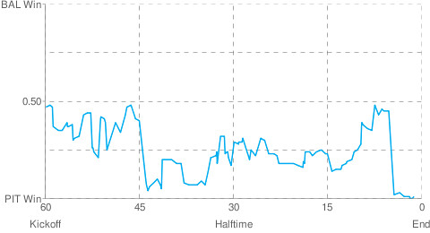
Both conference championships were remarkable games. And despite very different styles of play, both games followed the same plot line. One team seemingly dominated the entire game, only to see the underdog within striking distance of the upset with only a few minutes to play. Arizona fought off an unprecedented 2nd half comeback while Pittsburgh won in dramatic fashion late in the 4th quarter.

The Eagles trailed by 18 points late until scoring their first touchdown late in the 3rd quarter, making the score 24-13. Shortly before the score, they had a near-zero probability of winning. Just to tie, they would need 11 points while hoping to keep Arizona off the scoreboard for the rest of the game. Two more TDs later, and Philly miraculously had the lead 25-24. For a brief second, they actually broke above 0.50 WP before Arizona was able to score the last TD of the game, securing their first trip to the Super Bowl.


The AFC championship game's graph looks very similar. A see-saw battle in the first quarter gives way to a clear advantage for the home team. A comeback effort peaks midway through the 4th quarter but falls short.

Down by 2 points with about 7 minutes remaining, Baltimore forced a punt and gained possession on their own 40. But a boneheaded personal foul during the punt puts the ball back at the 14. Flacco's deep throw to Todd Heap gave the Ravens a 1st and 10 at their 32. With just 30 yards to go to get into Matt Stover's field goal range and a ticket to the Super Bowl, the Ravens had somehow battled back to a 0.45 WP. You might think that's high given the Steelers' phenomenal defense, and you might be right. But don't tell that to Tennessee fans.

Three plays later Steelers safety Troy Polamalu intercepted a Flacco pass and returned it 40 yards for a touchdown, making the score 23-14 and putting the game out of reach. In terms of pure leverage in getting to the Super Bowl, no other single play comes close. This was unquestionably the play of the year (so far).


Congratulations Steelers and Cardinals fans.

Win Probability Calculator

I've built a tool for calculating the Win Probability for a given state of a game, and it's now available on-line. I originally built it for myself to streamline analyses of kick/go-for-it type decisions. But I thought if I made the interface user friendly enough other people might find it useful or interesting too.

You just enter the score difference, time remaining, field position, and down and to go distance. The applet returns the win probability for the team with possession along with some other handy stats.

Here is an example of how I'd use it. Say a team is up by 3 points with 2 minutes remaining in the 4th quarter. They're pinned down at their own 2 yard line and are facing 4th and 9. Should they take the intentional safety and give the ball (on average) to the other team at their own 44? Or should they punt, saving the 2 points but handing the ball (on average) to the other team at your own 42, just outside of field goal range?

I'd look at it from the opponent's point of view since they'll have the ball. I'd enter -3 for score difference, 2:00 in the 4th for time remaining, opponent's 42 for field position, and 1st and 10. The resulting WP is 0.37 for the punt.

For the safety, I'd enter -1 for score difference, 2:00 remaining in the 4th, own 44 for field position, and 1st down and 10. The resulting WP is 0.38 for the safety.

Since we'd want the WP for the opponent to be as low as possible, the 0.37 for the punt is the better option, but just barely. The options aren't that far apart. So if the punter gets a bad snap or feels they're a good chance the punt would be blocked, he should just fall on the ball or run out of the endzone. Far better to take the safety in that situation than risk a blocked kick and an easy touchdown.

Another way to look at it uses the probabilities of scoring from each position. Let's make one assumption--With 2:00 remaining, there is plenty of time for the opponent to score from midfield, and if he does, there's not enough time left for you to answer.

If you chose to give up the intentional safety, your opponent has a 0.23 probability of scoring a TD, and a 0.16 of scoring a FG. Since the opponent only needs a FG, chances are he'd stop short of the TD once the FG is relatively assured, so the total chance of scoring is 0.39. Any score will beat you, so the 0.39 WP is very close to the 0.38 we got using the WP calculator directly.

The punt analysis tells a different story. From your 42 yard line, the opponent has a 0.32 probability of scoring a TD, which will beat you, and a 0.22 probability of scoring a FG, which will tie the game. The net WP for your opponent is therefore 0.32 + (0.5 * 0.22) = 0.43. This is a little off from the 0.37 WP we calculated directly. What causes the difference?

The direct WP calculations are based on actual game situations and results--that is, what did coaches really do, and what were the real outcomes? But the scoring probabilities are general and not specific to the particular game circumstances. The difference in the estimated WP suggests that coaches are too timid when behind by 3 at the end of the game. Once in FG position, they'll become very conservative and play for the tie rather than risk a turnover going for the TD and the win. It sounds reasonable...at first.

But a tie only gives you a 50/50 shot at winning, and turnovers--which would always cause a loss--occur far less than 50% of the time. A turnover of any type only occurs less that 12% of the time inside FG range (the 35). Coaches should press for the win as long as time and downs permit.

Ultimately, the safety might be the better option (0.39 vs 0.43) if coaches could actually be expected to play to win. But because coaches can usually be counted on to play for the tie, the punt is the slightly better option.

Weekly Roundup

Sabermetric Research points to this King Kaufman column in Salon.com. Kaufman takes sports writers to task for not appreciating advanced statistics. Sports writers and even some coaches are often dismissive of stats, and some even wear their ignorance as a badge of honor. Baseball is going through a quiet transformation based on advanced statistics. Stats are the cutting edge of the sport, and writers would do well to get on board. The way I see it, statistics is just a tool for learning from large sets of facts. Everyone relies on statistics one way or another. You can chose to do it well or do it poorly. Judging from the interest in this site and others, there is a sizable audience hungry for something other than the same old tired storylines we get from columnists and analysts.

Game theory could help improve the overtime problems in the NFL. This article talks about how to fairly divide something between two people. One of the best solutions is the I'll cut you choose method. So if two people splitting a piece of cake, one person would cut it in half, and the other picks which half he wants. The person cutting has an interest in making the division as fair as possible. Overtime could work the same way. The coin flip winner picks the yard line for kickoff, and the other team gets to chose whether to receive or kick. I don't think most traditionalists would like this idea, but neither team could complain about the outcome.

ZEUS chimes in on the Titans' decision to tie Ravens with a field goal instead of go for the first down on 4th and inches. Here was my take. But let me skip to the last chapter for everybody. It is almost always better to go for the first down, even up to 4th and 7 on a team's own side of the field in most cases. About the only times an NFL team should kick are on 4th and very long, or if time is expiring and the kick will win or tie the game.

ZEUS also thinks Coughlin was right to go for it against the Eagles. One thing about ZEUS, though--From what I can tell, the software is a simulation-based model. This means that it takes the current state of a game including score, time, field position, etc. and randomly simulates a game from that point forward. It does this 'millions' of times to estimate average win probabilities (that it calls game winning chance--GWC).

To me, this approach is fraught with problems. You'd have to model so many things so precisely to get a reliable result. The distributions of all possible play results for all the possible combinations of cirmcumstances simply could not be modeled with any reliability. You'd need to make a lot of assumptions, and the results are going to be very sensitive to those assumptions. It wouldn't be much different than playing out a game on Madden in auto-computer mode a million times. It just depends on the fidelity of the simulation. On the other hand, the advantage of this approach is that you can tweak the distributions to reflect specific team strengths and weaknesses.

Individual team abilities are mitigating considerations in kick or go-for-it decisions, but my take is that these factors are often overstated. Take the Ravens-Titans game. As I pointed out earlier this week, Baltimore had only scored on 2 of 10 possessions up until Fisher's decision to kick. That might indicate that the Titans defense could almost certainly count on stopping the Ravens offense. But the NFL average is 3 scores every 9 drives, not significantly different from 2 out of 10, and Baltimore went on to score to make it 3 out of 11. How much does under- or over-performance within a game predict performance later in a game? PFR took up that question and finds only about 25% of a team's under-performance in the first 3 quarters carries through to the 4th quarter.

Home field advantage (HFA) has been a focus of sports science for decades. We can quantify the strength of its effect pretty easily, but what are the causes? Is it travel fatigue, time zone change, weather, crowd noise, the shape of the field or cut of the grass, or referee bias? I think we now have pretty solid evidence that a large part of HFA comes from environmental familiarity.

The possible effect of general unfamiliarity was summed up well by a commenter: "From a psychological standpoint, performance could be subtlety infuenced due to players being in a somewhat unfamiliar environment due the small but cumulative effects of orienting to the new environment. This could be many things— the locker room, where the sun comes in over the stadium, the overall “feel.” All of these small distractions could influence performance–a performance that involves instantaneous decision making and physical reaction times. Research has shown that orienting to even environments that are somewhat unfamiliar influence memory, judgment, decison making, etc."

PFR took a look at HFA when opponents are familiar with each other. I thought that this might be what explains why HFA diminishes throughout a game. My suggestion was that because visitors are more familiar with environments when playing divisional opponents than when playing other opponents, we should see a reduced effect. And sure enough, that's exactly what we see. Division rivals not only have a reduced overall HFA, the quarter-by-quarter decline in HFA is shallower. To me, this is evidence that a good deal of HFA in the NFL is due to overall environmental familiarity. I think this is very interesting, and it comes mostly from loose collaboration from people who've never met. Twenty years ago, before the internet, research like this wouldn't be possible. We're not curing cancer, but it is interesting and useful. Further comments here.

Smart Football dissects the deep crossing route.

The Numbers Guy takes a look at rare NFL scores. The Chargers-Steelers 11-10 score is not the only unique score this year.

I really liked Jim Glass's comments about the distinction between the "best team" and "the campion."

Contributer jjbtnw looks at 3rd down and 6 situations. Should teams run more often?

Dean Jens takes a stab at modeling punting and field goal kicking.

Pacifist Viking has an excellent article about the classical correlation/causation fallacy. PV debunks a lot of analysis by Cold Hard Football Facts. But I do enjoy CHFF, but not because of the analysis there. The stats aren't always the soundest, but the analysis is much better than most other sites. The writing is excellent and I like the historical perspective they add. I wish I could write like that.

An article at NFL.com talks about which stats matter to coaches.

Sometime shortly I'll have a new Win Probability tool available. You can enter a game state and calculate the WP. I originally made it as a tool for myself when analyzing things such as 4th down decisions, but thought other people might find it interesting too. So I spiffed up the interface and will have it up and running soon.