Leading Indicators 2

"Anti-Predictors"

In the last post I compared the results of two regression models. The first model estimated current year wins based on current year stats. The second model predicted next year’s wins based on last year’s stats. The comparison of the regression results revealed how well various team stats persist from year to year as predictors of team wins.

I found that the stats that persisted from season to season as a predictor of wins were offensive running efficiency (36%), team penalties (52%), and defensive forced fumble rates (45%). I also found two stats that could be considered anti-predictors. Offensive and defensive interception rates both reverse their direction of prediction across seasons. In other words, a low offensive pass interception rate for a team in one year foretells fewer wins the following year, all other things being equal.

This is a confusing result, to say the least. One possible explanation is random coincidence--the stats may show a connection only by chance. However, the significance of the offensive interception coefficient was 0.07 and the defensive interception coefficient was 0.09. As I wrote earlier, the FDA might not approve heart medication based on trials with marginal significance levels, but it is still highly unlikely that both coefficients suffer from statistical Type I errors. After all, we’re not splitting the atom here. We’re just talking about football.

In the last post I wrote, “My theory is that we are witnessing regression to the mean. For many teams, interception rates have a lot of variance due to luck. So a team that is unlucky with interceptions one year is not likely to be as unlucky the next year, [and vice versa]. That could partially explain the reversed signs. Another possibility is that teams systematically swing from high to low interception rates from one season to the next, something I strongly doubt.”

A friend at work suggested I actually look at teams, their players, and what happened that might cause such a result. (What? There’s more to football than statistics?) I couldn’t bring myself to qualitatively analyze what might be going on, but he did inspire me to dig a little deeper.

Below is a list teams that demonstrated the trend of impressive interception rates one year, followed by a severe drop-off in wins the next. The average for both offensive and defensive interception rates is 0.32.

Year	Team	Wins	Next Wins	O Int Rate	D Int Rate
2002	TB	12	7	0.018	0.061
2002	OAK	11	4	0.016	0.037
2003	TEN	12	5	0.018	0.038
2003	KC	13	7	0.022	0.044
2004	PHI	13	6	0.020	0.031
2005	TB	11	4	0.029	0.036
2004	NYJ	10	4	0.025	0.038
2005	JAX	12	8	0.012	0.039
2003	SF	7	2	0.029	0.045
2005	CIN	11	8	0.026	0.060
2004	HOU	7	2	0.030	0.042
2002	ATL	9	5	0.025	0.047
2003	MIA	10	4	0.042	0.042
2005	DEN	13	9	0.015	0.033
2005	WAS	10	5	0.023	0.030
2004	BUF	9	5	0.037	0.049
2004	SD	12	9	0.018	0.038
2003	STL	12	8	0.038	0.047
2004	NE	14	10	0.029	0.037
2004	BAL	9	6	0.024	0.042
2005	SEA	13	9	0.021	0.028
2004	NO	8	3	0.030	0.024
2004	GB	10	4	0.032	0.015

These teams all exhibited a notably better than average interception rate on either offense or defense, only to suffer a dramatically worse record the next year.

Below is the list of teams that exhibit the opposite trend, no matter how slight. They exhibited better than average interception rates, then improved their record the following year.

Year	Team	Wins	Next Wins	O Int Rate	D Int Rate
2005	TEN	4	8	0.024	0.019
2005	NYJ	4	10	0.032	0.045
2004	NYG	6	11	0.027	0.030
2002	KC	8	13	0.027	0.029

Whatever the reason for the phenomenon, it appears real. It might be summed up by "Live by the interception, die by the interception." If a team wins a lot of games based on superior offensive (low) or defensive (high) interception rates, it tends to be extremely difficult to repeat, and that team will very probably not win as many games the following year.

In the next post, I'll apply the leading indicators to the team stats from 2006. I'll list how each team can be expected to benefit (or suffer) in 2007 from the leading indicators of NFL wins.

Leading Indicators 1

Predicting team win totals before the season begins is a very inexact science. Although I’ve predicted the win total of all the teams for 2007 based on last year’s performance stats, the estimates are fairly vague. The reason for the lack of confidence is that team performance in one area does not necessarily remain consistent across seasons. But we can measure which team performance predictors do tend to persist from year to year. The stats that endure as predictors of following year wins can be considered leading indicators.

I ran two regressions. The first was my usual model using efficiency stats to estimate team wins for the year in question. The second model used the same efficiency stats to estimate team wins for the next year. In other words, it used 2002 stats to predict 2003 wins. The data set included the ’02-’06 seasons. By comparing the results, we can see which stats tend to be consistent predictors from year to year.

The efficiency stat predictors were converted into standardized variables. This way, they can be directly compared to each other in terms of their relative importance in estimating wins. The % Persist column calculates the proportion of predictive power retained from one year to the next. It was calculated by dividing each coefficient of the next year model by the current year model, then adjusting for the r-squared of each regression.

Same Yr Wins				Next Yr Wins
VARIABLE	COEF	SIG.		VARIABLE	COEF	SIG.		% Persist
O Pass	1.22	0.00		O Pass	0.42	0.11		9.4
D Pass	-1.11	0.00		D Pass	-0.01	0.97		0.2
O Run	0.42	0.00		O Run	0.56	0.01		36.0 *
D Run	-0.16	0.23		D Run	0.00	0.99		-0.5
Penalties	-0.23	0.07		Penalties	-0.44	0.09		52.6 *
O Fum	-0.42	0.01		O Fum	-0.05	0.83		3.5
D FFum	0.47	0.00		D FFum	0.78	0.00		45.3 *
O Int	-0.32	0.03		O Int	0.40	0.07		-34.2 ?
D Int	0.60	0.00		D Int	-0.34	0.09		-15.5 ?
r-squared	0.75			r-squared	0.20

The results of the first regression produced expected results. It estimated present year wins very well (r-squared=0.75), with all variables significant. The second regression, which predicted following year wins, was expectedly much weaker (r-squared=0.20), but it revealed which stats endure from year to year as predictors of team wins.

It shows that offensive run efficiency, team penalties, defensive forced fumbles, and interceptions thrown are relatively persistent predictors of following year wins. Defensive pass and run efficiencies are not consistent predictors.

I adjusted the coefficients in each model by their respective model’s r-squared values. Then I divided the second (next year) model’s coefficients by the first. This tells us the percent of predictive value of each stat that survives from one season to the next. In other words, I calculated how much of each stat’s predictive power survives the off-season to help predict next year’s wins. For example, only 9% of the predictive power of offensive pass efficiency endures.

We see that the stronger persisting stats are offensive running efficiency (36%), team penalties (52%), and defensive forced fumble rate (45%).

Notice that the interception rate stats also show persistence (45%, 34%), but that the signs of the coefficients are reversed between models. This means that these stats could be considered ANTI-predictors. In other words, a low offensive pass interception rate in one year signifies fewer wins the following year. This is unexpected and could be just due to their marginal significance. But although p-values of 0.07 and 0.09 may not good enough for the FDA to approve heart medication, it’s still extremely likely that the results signify something is at work.

My theory is that we are witnessing regression to the mean. For many teams, interception rates have a lot of variance due to luck. So a team that is unlucky with interceptions one year is not likely to be as unlucky the next year. That could partially explain the reversed signs. Another possibility is that teams systematically swing from high to low interception rates from one season to the next, something I strongly doubt. Otherwise, I’m at a loss to explain this result.

Examining the results as a whole, including the lack of persistence in defensive stats and the anti-prediction of interception stats, indicate that defensive performance, and secondary performance in particular, is not persistent from year-to-year as an indicator of team win totals. It is not reliable as an indicator of wins from season to season compared to other facets of the game.

Continue reading part 2 of this article.

Median Rushing Yards

What's the difference between these two situations?

1. On 1st and 10 from the opponent's 30, a RB gets a handoff and breaks free for a 30 yd TD.

2. On 1st and 10 from his own 30, a RB gets a handoff and breaks free for a 70 yd TD.

In both plays, the RB read the blocks and made the moves necessary to break into the open field. In both plays the RB's speed and agility beat the safeties. But the difference of 50 yds is basically statistical trash because in situation #1, the RB likely could have kept running for another 50 yds.

In rating running ability, I've previously suggested the use of median statistics rather than average statistics. When we want to know how good a team's running game is, or how good a RB is, we want to know the central tendency of the team or player. The statistical mean is only one way of looking at central tendency. Median can often be more useful. Averages are often distorted by a very few outlier inputs.

Consider this fictitious example examining the central tendency of college dropouts who live in Redmond, WA. Let's say there are 5,000 college dropouts in Redmond, Washington, and each make $30,000/yr except this one guy named Gates. He makes $20 billion/yr. The average salary of a college dropout in Redmond is over $4 million/yr. So if I'm a student in Redmond I should skip class tomorrow, right? $4 million/yr might be the average, but it's not the central tendency and it's virtually useless information.

Which player would you rather have on your team? A RB who gets at least 4 yds on every carry, or a RB who gets 29 1-yd runs and one 91-yd run? Both players average 4 yds/carry. The first player's median rush is 4 yds and the second player's is 1 yd. It's an extreme example, but it illustrates my point. Consistency has its value.

Here are a list of the top runners of 2006 sorted in order of their percentage of runs >4 yds. It's interesting to compare to their average yds/rush, their total yards, and other stats. (Ties are broken by % of carries > 3 yds.)

RB	TEAM	4YD PCT	ATT	YDS	AVG	TD	FUM	LST	TD/ATT%
Norwood	ATL	57	99	633	6.4	2	0	0	2.0
Addai	IND	54	226	1081	4.8	7	2	2	3.1
Westbrook	PHI	50	240	1217	5.1	7	1	1	2.9
Washington	NYJ	50	151	650	4.3	4	1	1	2.6
Betts	WAS	48	245	1154	4.7	4	4	2	1.6
Barber	NYG	47	327	1662	5.1	5	3	1	1.5
Barber	DAL	47	135	654	4.8	14	0	0	10.4
Tomlinson	SD	46	348	1815	5.2	28	2	1	8.0
Gore	SF	46	312	1695	5.4	8	5	5	2.6
Jones	CHI	46	296	1210	4.1	6	1	1	2.0
McAllister	NO	46	244	1057	4.3	10	2	1	4.1
Vick	ATL	46	123	1039	8.4	2	4	2	1.6
Jones-Drew	JAX	46	166	941	5.7	13	1	1	7.8
Dillon	NE	46	199	812	4.1	13	2	2	6.5
Jackson	STL	45	346	1528	4.4	13	2	1	3.8
Dayne	HOU	45	151	612	4.1	5	1	0	3.3
Brown	MIA	44	241	1008	4.2	5	4	2	2.1
McGahee	BUF	44	259	990	3.8	6	4	2	2.3
Fargas	OAK	44	178	659	3.7	1	1	0	0.6
Benson	CHI	44	157	647	4.1	6	0	0	3.8
Henry	TEN	43	270	1211	4.5	7	3	1	2.6
Williams	TAM	43	225	798	3.5	1	2	2	0.4
James	ARI	42	337	1159	3.4	6	3	3	1.8
Foster	CAR	42	227	897	4.0	3	3	2	1.3
Maroney	NE	42	175	745	4.3	6	1	1	3.4
Rhodes	IND	42	187	641	3.4	5	2	2	2.7
Taylor	MIN	41	303	1216	4.0	6	4	3	2.0
Taylor	JAX	41	231	1146	5.0	5	2	1	2.2
Bell T.	DEN	41	233	1025	4.4	2	3	3	0.9
Bell M.	DEN	41	157	677	4.3	8	1	0	5.1
Johnson	KAN	40	416	1789	4.3	17	2	2	4.1
Johnson	CIN	40	341	1309	3.8	12	6	2	3.5
Lewis	BAL	40	314	1132	3.6	9	4	2	2.9
Jones	DAL	40	267	1084	4.1	4	1	1	1.5
Droughns	CLE	40	220	758	3.4	4	5	4	1.8
Parker	PIT	39	337	1494	4.4	13	6	4	3.9
Dunn	ATL	39	286	1140	4.0	4	1	0	1.4
Alexander	SEA	39	252	896	3.6	7	5	3	2.8
Morris	SEA	39	161	604	3.8	0	1	1	0.0
Green	GB	37	266	1059	4.0	5	2	2	1.9
Jones	DET	36	181	689	3.8	6	4	4	3.3

I'm not suggesting average rushing is worthless, just that it is only part of the story.

Rushing TDs and Passing

Rushing touchdowns are the holy grail of fantasy football. They're the most scarce scores. Everyone starts the draft by picking 2 RBs (except the guy who always takes Peyton Manning first).

Rushing TDs are a product of a great running game, right? That's only half true. Rushing TDs have just as much to do with a good passing game as a running game. That's not shocking news to most serious football fans. No team can run the ball all the way down the field without at least a few pass completions. But the extent to which rushing TDs are dependent on the passing game may surprise some.

Rushing TDs correlation with:
---------------------------------
Team Yds/Rush 0.50
Team Yds/Pass Att 0.46

Going a little deeper, we can run a quick regression using rushing and passing efficiency (including sack yards) to estimate rushing TDs. Interceptions are a big part of the passing game--teams that throw a lot of INTs would be expected to limit their opportunities for rushing TDs. So I'll include interception efficiency in the model. I'll also use standardized variables so we can directly compare the relative importance of each variable. Based on data from the '02-'06 seasons, the regression produces the following results:

VARIABLE	COEFFICIENT	STDERROR	T STAT	P-VALUE
const	13.51	0.35	38.88	0.00
Z RUN AVG*	2.56	0.35	7.27	0.00
Z PASS EFF*	2.16	0.39	5.54	0.00
Z INT RATE	-0.34	0.39	-0.88	0.38
R-squared	0.42

The coefficient of RUN AVG (yds/rush) is 2.56 while the coefficent of PASS EFF (yds/att) is 2.16, which tells us that a good passing game is almost as important as a good running game in producing rushing TDs.

But if we consider the importance of INT RATE (INTs/att), we see that the importance of the passing game nearly equals that of the running game in producing rushing TDs (2.56 vs. 2.50).

So if other teams in your league have already picked up Stephen Jackson and Larry Johnson, or if you're looking for a #3 RB to fill the gap when LT has a bye in week 7, then look for an overlooked RB on a team with a decent passing game.

Luck: Epilogue

Coincidentally, as I was posting the results of my look at the amount of luck in NFL games, Phil Birnbaum posted this at his site. He was sharing a paper he did a while back about how "truly" good an MLB team is that wins 100 games. If some games are won on merit, and some by luck, then his calculations say the average 100 game winner won by luck 7 games more than they merited based on the their talent level. In other words, 100 game winners are probably both good and lucky.

But even more interesting was another tidbit Phil linked to. If you follow the references, you land here on Tom Tango's site. He's another accomplished sabermetrician. He approached the question of luck in sports outcomes far more elegantly than I did.

There, he works through his math calculating how many games are required for a sports league to produce the "true" best team on top of the standings. For MLB he says it's 69 games, and for the NFL it's 12 games.

Along the way, Tango articulates his theory. Regarding the distribution of win-loss records, the observed variance is: variance(observed) = varance(true) + variance (luck). Since we know the variance of the observed distribution (SD^2), and we know the variance of luck from the binomial distribution (p=0.5, n=16), we can solve for variance (true), which is the variance in team records based on merit.

I'm not sure what to think about his method. His theory assumes the "true" distribution (what I call pure-skill) is narrower than the observed distribution. Then luck acts on the true distribution to widen it.

But my simulations show that the distribution of a pure merit league is much wider than either the observed or the luck distributions. So I'm not sure how to interpret his theory.

On another note, I reran my simulation against the 96-01 NFL seasons. The scheduling system was a little different then, but the effect should be minimal. The simulation maximized its goodness-of-fit at 51% luck, which is pretty much what I found for the 02-06 seasons.

Upcoming posts include a look at YAC stats and how they affect QB stats, and a look at what really produces rushing TDs--something for the fantasy football fans out there.

Luck and NFL Outcomes 3

This is the third and final post of an article discussing the amount of luck in determining outcomes in the NFL. In the first post, I compared the actual distribution of team win-loss records over the past five seasons with an idealized pure luck distribution. I found that only 78 out of 160 actual season records (48%) differed from what we’d expect if the NFL were determined completely by luck.

In the second post, I compared the actual distribution with an idealized distribution of records in a theoretical league governed by “pure skill.”

In this post, I will unify the three distributions--actual, luck, and skill--into one algorithm. The resulting equation reveals the proportion of NFL games in which the deciding factor is luck and not the camparitive strength of each opponent.

LUCK, SKILL, AND OBSERVED

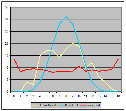
The chart below is a histogram of the pure binomial distribution, the simulated pure-skill (zero luck) distribution, and the actual distribution of NFL records since the '02 expansion. (Pure luck is blue, actual is yellow, and pure skill is red.)

When I first examined the three distributions together, I was struck by how the actual distribution appeared to split the difference between the luck and skill distribution. The actual records appear to be some sort of combination of the luck and skill distributions. To me, it looked as if the pure-luck binomial distribution was pressed into a flatter and wider distribution by skill.

LUCK/SKILL SYNTHESIS

It dawned on me to create another simulation, one that synthesized the pure-luck and pure-skill distributions together in varying degrees. (10% luck/90% skill, 20% luck/80% skill, etc.) Basically, the luck% variable determined a percentage of games (chosen at random) to be decided by pure luck, essentially a coin flip. The remainder of the games were credited to the superior team. The simulation algorithm looked like this:

If rand() < %luck, then game outcome = pure luck, else game outcome = win by the better team

I varied the %luck value between 0 and 1, re-running the simulation. Here are some representative win distributions (legend is in %luck):

Next I overlayed the actual distribution.

PROPORTION OF LUCK IN NFL OUTCOMES

Then I varied the %luck value until it maximized the goodness of fit between the actual distribution and the synthesized distribution. At 52.5% luck, the theoretical distribution is statistically indistinguishable from the actual distribution (chi-square goodness of fit p=0.94). This means it is 94% probable that the discrepancies between the synthesized simulation and the actual observations are merely due to sample error.

THEORETICAL MAXIMUM PREDICTION RATE

I will be very careful in stating what conclusion I draw from this exercise. The actual observed distribution of win-loss records in the NFL is indistinguishable from a league in which 52.5% of the games are decided at random and not by the comparative strength of each opponent.

I admit 52.5% seems very high. But keep in mind, that half of the time, the better team wins by luck. In other words, half the time our prediction models are correct by chance, just like a monkey picking winners would be. If the 52.5% figure is correct, the best any prediction model could do is:

0.50 + 0.525/2 = 0.76

So 76% correct would be the theoretical ceiling for NFL game prediction models. This is consistent with the various computer models as well as odds makers. It is also consistent with our intuitive experience--upsets seem happen about a quarter of the time. Sometimes a model (or a person) can predict at better than a 76% correct rate, but anything above that would be...by luck.

I also posted a follow up to this series of articles here.

A Definition of Luck in Sports

This post is a little different than my others. I think it would serve my luck research well if I take some time to explain what I define as luck.

Luck is just my shorthand for a random process, and I admit using the word luck may be misleading. A random process is merely one in which the outcome cannot be controlled, and that each possible outcome has an equal chance of occurring. The accumulation of effects of several random processes results in a normal distribution, like balls bouncing down a Pachinko board.

Flipping a coin is not luck in a strict technical sense. It is dependent on its original position, the rate of spin imparted, the height of the toss, etc. But the outcome cannot be controlled, and each possible outcome is equally likely. Hence, it is indistinguishable from a true random process--what could just as well be called luck. In football, as in any sport, there are many processes similar to a coin flip.

One example would be a punt that first lands on the 5 yard line. Does it die on the 2 yard line or will it bounce into the endzone for a touchback? Once the punt hits the ground it is no longer under the influence of the punter in any way. Over time the randomness will average out and good punters will tend to prevent more touchbacks. But where this one punt lands today, in this one game, right now, is partly random.

Randomness can play a very strong role in the outcome of any single game. Consider a baseball game between a team and its perfect equal in every measure. In this evenly matched game, each team hits 9 singles. Team A happens to get its singles within 3 innings, then goes hitless for 6. Each inning of 3 singles produces 1 run. Team B's 9 singles happen to be spread across 9 innings, resulting in zero runs. Team A wins 3-0, although each team performed equally well.

The total number of singles produced by a team is controlled by the interaction of skills between batters, pitchers, and defense--certainly not luck. But, when the singles occur and how they are bunched cannot be controlled, and their distribution is equally likely throughout the game. Batters have zero ability to chose when their hits occur. If they did, everyone's average with "runners in scoring position" would be much higher. Therefore, when the hits occur is indeed random, and consequently, a sizable part of the outcome of a any single game is random.

It's why the Devil Rays sometimes beat the Yankees. They weren't the better team that day. They just benefited more from a random dispersion of events more than their opponents did.

Baseball managers have understood this effect for generations. This is partly why a team's lineup is usually constructed with its best batters bunched together in order. It maximizes the probability that hits will come in bunches. This technique skews the random distribution positively, but does not reduce the randomness of the process itself.

Football is very different from baseball, but the bunching effect exists on the grid-iron too. Scoring drives are not just dependent on achieving several first downs, but on achieving consecutive first downs. The total number of first downs earned is determined by the relative strength of each team, but how dispersed they are is random. So part of the game outcome is due to the teams' comparative strength, and part is due to a random process.

Randomness is an essential part of the physical universe. Perhaps instead of luck I should use the word chance or randomness. Luck implies superstition, to which I certainly do not subscribe. I do not believe one side or the other enters a contest with some Goddess of Luck smiling its side. Instead of saying "the Giants had luck on their side today," I should say "the cumulative outcome of uncontrolled random processes favored the Giants in this game."

But if you don't buy into randomness--what I call luck--you're in good company. Einstein denied it too. His feelings were summed in his quote "God does not play dice with the universe." Randomness offended his sense of a rational universe, just as many sports fans are offended by the role luck plays in sports. Unfortunately, his refusal to accept it brought his research to a dead end. Subsequent research led to quantum physics, which confirms randomness as a fundamental property of reality.

Lastly, if you don't believe in randomness you must not be reading this. One of the greatest human technological advances in history requires randomness to exist and be quantifiable--the microprocessor.

Luck and NFL Outcomes 2

This is a continuation of an article discussing the amount of luck in determining outcomes in the NFL. In the last post, I compared the actual distribution of team win-loss records over the past five seasons with an idealized pure luck distribution. I found that only 78 out of 160 actual season records (48%) differed from what we’d expect if the NFL were determined completely by luck. In this post, I will compare the actual distribution with an idealized distribution of records in a theoretical league governed by “pure skill.”

A PURE SKILL LEAGUE

A pure skill league would be one in which the better team always won. There would be no upsets. I originally had great difficulty imagining what the distribution of such a league would look like. The very best team would always win 16 games, and the very worst team would always win zero. I suspected that the distribution would be flat in between the two extreme cases so there would be the same number of 3-13 teams as there were 4-12 teams as there were 5-11 teams, etc. I thought the resulting distribution would resemble a trapezoid. I was close.

I created a simulation to determine exactly what a pure-skill distribution would look like. In the simulation there are 32 teams that play sixteen games. The schedule for each team is assigned just as it is in the NFL. Each team plays three teams twice, then plays 10 other games against extra-divisional opponents. Each simulated year creates a unique schedule.

Each year, team #1 is the very best team and #32 is the very worst team. It does not matter which team is #1 or #2 because we merely need to see the distribution of records, not identify which specific teams earned those specific records. Each year there is a very best and a very worst team, and every other team is slotted in between. In the pure-skill league, whenever a team plays an inferior opponent it wins, and whenever it plays a superior opponent it loses. Luck is therefore never a factor.

[Before anyone starts trying to poke holes in the simulation, keep in mind this is a theoretical ideal only, and does reflect all the complications of injuries or weather advantages, etc., nor does it need to. Also, when you see the next post, you will see with your own eyes how realistic the simulation really is.]

The table below gives an abbreviated sample of how I visualized a league schedule in which wins are determined by team strength alone. The team rank column signifies the relative strength of the team. The next column indicates the probability that any given opponent is better than the listed team. The next columns list the opponents for the team in the simulated season. To calculate the wins for each team, I simply counted how many simulated opponents were worse than the listed team.

Team Rank	Prob. Opp. is Better	Div Gm1	Div Gm2	Div Gm3	…	Gm16	Wins
1	0.00	27	27	32	…	25	16
2	0.03	2	2	7	…	2	16
3	0.06	18	18	25	…	14	15
…	…	…	…	…	…	…
31	0.97	30	30	17	…	23	1
32	1.00	12	12	2	…	20	0

Thousands of simulated seasons were played out and the resulting distribution is illustrated below.

The distribution shows that about 8% of records result in undefeated season, and the same share results in a winless record. Between 1 and 15 wins, there is an even share of results, each at about 6%.

The distribution appears to be an inverted trapezoid. The extra cases of 0-win and 16-win teams are a result of the schedule format. Because there are 32 teams, and 16 games against 13 opponents, some teams will not play each other each year. So the 31st best team may not get to play the 32nd best team and would end up winless. The #2 team may not have to face the #1 team and would have 16 wins. The same would go for the #3 team, but it would be slightly less likely.

COMPARING PURE SKILL AND OBSERVED

Now let’s look at how the pure skill distribution compares to the actual observed distribution of NFL regular season records over the past 5 years. The two distributions are plotted below on the same scale.


The two distributions are obviously different. The goodness-of-fit chi-square is conclusive as well (p=1.0E-10). But there are some similarities. For example, the actual distribution has somewhat of a plateau through the middle of the range, between 4 and 10 wins. We also see that it is not unusual to see irregularities in the distribution, even for the idealized simulation conducted over many seasons.

Now examine all three distributions together. The actual, pure luck, and pure skill distributions are illustrated below. I’m guessing most readers will notice the same thing I did.

In the third and final part of this article, I’ll discuss what all these distributions have in common, and how I mathematically calculated the relationship between them. The result reveals what proportion of NFL game outcomes are decided by luck, and what proportion is decided by the relative strength of each team.