
 For every series beginning with a 1st down and 10 in the NFL, an offense achieves another 1st down (including scoring a TD) 66% of the time. So if an offense is to be graded on a 1st down play, it should at least gain enough yards so that they have at least the same probability of sustaining the drive or scoring. In this article, I’ll begin a discussion of utility in football by examining the break even point in a series of downs. In other words, what would you rather have, a 1st and 10 or 2nd and 7? What about 2nd and 6? 5?
When any team has the ball, it's typically trying to sustain a drive. It would be nice if they threw a 50 yard bomb for a touchdown, but usually their most immediate priority is to retain possession by getting a 1st down. One way to measure a play’s success is by how much it improves or impairs a team’s probability of getting there.
The graph below illustrates the probability of eventually achieving a 1st down in a current series given various ‘to go’ distances on 2nd down and 3rd down. Data is from all regular season plays from 2002 through 2007.
We can see that the break even point for 2nd down is 5.5 yards. In other words, a team (whose purpose is to get a 1st town) should prefer a 2nd down and 5 to a 1st and 10, but it should prefer a 1st and 10 to 2nd and 6.
For 3rd down, the break even point is at 1.5 yards. A team should prefer a 1st and 10 to any other 3rd down situation 2 yards or longer. This was a little surprising to me. I expected the break even point to be around 3rd and 3 or 4.
We can also compare other situations. Consider a team with a 2nd and 8. The chance of getting a first down on their current series is 57%. To break even in terms of 1st down probability, they need to gain at least 5 yards to have a 3rd down and 3. In fact, the two probability curves are generally separated by 5 yards, between the usual situation of 10 yards to go and 2 yards to go.
Five yards appears to be the magic number. Unless a team gains 5 or more yards on a given play, it’s a setback in terms of 1st down probability.
Carroll, Parmer, and Thorn, the authors of The Hidden Game of Football, established a measure of football play success in similar terms. In their system, if an offense gains at least 4 yards on 1st down, the play is considered a success. On 2nd down, the play is considered successful if it gains half the remaining distance to the first down marker. And 3rd down is only considered a success if it gains a 1st down. This may sound familiar to some readers because the Football Outsiders blog applies this same system, with limited modifications, in their DVOA scheme.
According to the actual probabilities of gaining a first down, however, this system isn’t always consistent. An offense needs 5 yards on 1st down, not 4, to break even in terms of first down probability. Also, gaining half the yards remaining on 2nd down often leaves a team worse off than it was before the play began.
Getting anything less than a 1st down on 2nd and 4 or less leaves a team with a lower probability. On 2nd down and 7, a team’s chance of getting a 1st down is 62%. Gaining half the remaining yards leaves the offense at 3rd and 3.5 yards, which yields a 1st down 54% of the time. They’d need to be inside 3rd and 2 to break even.
This is only one way to measure success in football. There are others, such as expected points and win probability. I’ll take a look at those methods in upcoming articles.
First Down Probability
Drunkards, Light Posts, and the Myth of 370
 Running back overuse has been a hot topic in the NFL lately, partly because of Football Outsiders' promotion of their "Curse of 370" theory. In several articles in several outlets, including their annual Prospectus tome, they make the case that there is statistical proof that running backs suffer significant setbacks in the year following a season of very high carries. But a close examination reveals a different story. Is there really a curse of 370? Do running backs really suffer from overuse?
Football Outsiders says:
"A running back with 370 or more carries during the regular season will usually suffer either a major injury or a loss of effectiveness the following year, unless he is named Eric Dickerson.
Terrell Davis, Jamal Anderson, and Edgerrin James all blew out their knees. Earl Campbell, Jamal Lewis, and Eddie George went from legendary powerhouses to plodding, replacement-level players. Shaun Alexander struggled with foot injuries, and Curtis Martin had to retire. This is what happens when a running back is overworked to the point of having at least 370 carries during the regular season."While it's true that RBs with over 370 carries will probably suffer either an injury or a significant decline in performance the following year, the reason is not connected to overuse. What Football Outsiders calls the 'Curse of 370' is really due to:
Injury Rate Comparison
In the 25 RB seasons consisting of 370 or more carries between the years of 1980 and 2005, several of the RBs suffered injuries the following year. Only 14 of the 25 returned to start 14 or more games the following season. In their high carry year (which I'll call "year Y") the RBs averaged 15.8 game appearances, and 15.8 games started. But in the following year ("year Y+1"), they averaged only 13.0 appearances and 12.2 starts. That must be significant, right?
The question is, significant compared to what? What if that's the normal expected injury rate for all starting RBs? If you think about it, to reach 370+ carries, a RB must be healthy all season. Even without any overuse effect, we would naturally expect to see an increase in injury rates in the following year.
In retrospect, comparing starts or appearances in such a year to any other would distort any evaluation. This is what's known in statistics as a selection bias, and in this case it could be very significant.
We can still perform a valid statistical analysis however. We just need to compare the 370+ carry RBs with a control group. The comparison group was all 31 RBs who had a season of 344-369 carries between 1980 and 2005. (The lower limit of 344 carries was chosen because it produced the same number of cases as the 370+ group as of 2004. Since then there have been several more which were included in this analysis.)
Fortunately there is a statistical test perfectly suited to comparing the observed differences between the two groups of RBs. Based on sample sizes, differences between means, and standard deviation within each sample, the t-test calculates the probability that any apparent differences between two samples are due to random chance. (A t-test results in a p-value which is the probability that the observed difference is just due to chance. A p-value below 0.05 is considered statistically significant while a high p-value indicates the difference is not meaningful.) The table below lists each group's average games, games started, and the resulting p-values in their high-carry year and subsequent year.G Year Y G Year Y+1 GS Year Y GS Year Y+1 370+ Group 15.8 13.0 15.8 12.2 344-369 Group 15.8 14.0 15.4 12.6 P-Value 0.62 0.68
The differences are neither statistically significant nor practically significant. In other words, even if the sample sizes were enlarged and the differences became significant, the difference in games started between the two groups of RBs is only 0.4 starts and 1.0 appearances. RBs with 370 or more carries do not suffer any significant increase in injuries in the following year when compared to other starting RBs.
Regression to the Mean
The 370+ carry group of RBs declined in yards per carry (YPC) by an average of 0.5 YPC compared to a decline of 0.2 YPC by the 344-369 group. This is an apparently statistically significant difference, but is it due to overuse?
Consider why a RB is asked to carry the ball over 370 times. It's fairly uncommon, so several factors are probably contributing simultaneously. First, the RB himself was having a career year. He was probably performing at his athletic peak, and coaches were wisely calling his number often. His offensive line was very healthy and stacked with top blockers. Next, his team as a whole, including the defense, was likely having a very good year. Being ahead at the end of games means that running is a very attractive option because there is no risk of interception and it burns time off the clock. Additionally, his team's passing game might not have been one of the best, making running that much more appealing. And lastly, opposing run defenses were likely weaker than average. Many, if not all of these factors may contribute to peak carries and peak yardage by a RB.
What are the chances that those factors would all conspire in consecutive years? Linemen come and go, or get injured. Opponents change. Defenses change. Circumstances change. Why would we expect a RB to sustain two consecutive years of outlier performance? The answer is we shouldn't. Running backs with very high YPC will get lots of carries, but the factors that helped produce his high YPC stats are not permanent, and are far more likely to decline than improve.
If I'm right, we should see a regression to the mean in YPC for all RBs with peak seasons, not just very-high-carry RBs. The higher the peak, the larger the decline the following year. And that's exactly what we see in the data.
The graph above plots RB YPC in the high-carry year against the subsequent change in YPC. The blue points are the high-carry group, and the yellow points are the very-high-carry group. Note that there is in fact a very strong tendency for high YPC RBs to decline the following year, regardless of whether a RB exceeded 370 carries.
Very-high-carry RBs tend to have very high YPC stats, and they naturally suffer bigger declines the following season. 370+ carry RBs decline so much the following year simply because they peaked so high. This phenomenon is purely expected and not caused by overuse.
Statistical Trickery
Why did Football Outsiders pick 370 as the cutoff? I'll show you why in a moment, but for now I'm going to illustrate a common statistical trick sometimes known as multiple endpoints by proving a statistically significant relationship between two completely unrelated things. I picked an NFL stat as obscure and random as I could think of--% of punts out of bounds (%OOB).
Let's say I want to show how alphabetical order is directly related to this stat. I'll call my theory the "Curse of A through C" because punters whose first names start with an A, B, or C tend to kick the ball out of bounds far more often than other punters. In 2007 the A - C punters averaged 15% of their kicks out of bounds compared to only 10% for D - Z punters. In fact, the relationship is statistically significant (at p=0.02) despite the small sample size. So alphabetical order is clearly related to punting out of bounds!
Actually, what I did was sort the list of punters in alphabetical order, and then scanned down the column of %OOB. I picked the spot on the list that was most favorable to my argument, then divided the sample there. This trick is called multiple endpoints because there are any number of places where I could draw the dividing line (endpoints), but chose the most favorable one after looking at the data. Football Outsiders used this very same trick, and I'll show exactly how and why.
The graph below plots the change in yards per carry (YPC) against the number of carries in each RB's high-carry year. You can read it to say, a RB who had X carries improved or declined by Y yards per carry the following year. The vertical line is at the 370 carry mark.
Note the cluster of RBs highlighted in the top ellipse with 368 or 369 carries. They improved the following year. Now note the cluster of RBs highlighted in the bottom ellipse. They had 370-373 carries and declined the next year.
If we moved the dividing line leftward to 368 then the very-high-carry group would improve significantly. And if we moved line rightward to 373, then the non-high carry group would decline. Either way, the relationship between high carries and decline in YPC disappears. There is one and only place to draw the dividing line and have the "Curse" appear to hold water.
To be fair to Football Outsiders, they have recently admitted there is nothing magical about 370. A RB isn't just fine at 369 carries, and then on his 370th his legs will fall off. But unfortunately, that's the only interpretation of the data that supports the overuse hypothesis. If you make it 371 or 369, the relationship between carries and decline crumbles. It's circular to say that 370 proves overuse is real, then claim that 370 is only shorthand for the proven effect of overuse.
As Mark Twain (reportedly) once said, "Beware of those who use statistics like a drunkard uses a light post, for support rather than illumination."
Ideas, data, quotes, and definitions from Doug Drinen, PFR, Maurlie Tremblay, and Brian Jaura.
Why the Chargers Defense Will Decline in '08
 The San Diego Chargers led the NFL last year with +24 net turnovers. After starting the season slowly with a 1-3 record, they went on to finish 11-5, including ending the regular season on a 6-game win streak. The streak was in large part due to their phenomenally high defensive interception rate. Led at CB by second year sensation Antonio Cromartie who topped the league with 10 picks, San Diego posted an amazing 5.4% interception rate. Unfortunately for Charger fans, interception rates like the this just don't repeat themselves. I'll illustrate exactly why we shouldn't expect the Chargers to duplicate their dominant performance in 2008.
Previously, I've found that team defensive interception stats are extremely inconsistent. The more consistent a stat is, the more likely it is due to a repeatable skill or ability. The less consistent it is, the more likely the stat is due to unique circumstances or merely random luck. In other words, interceptions are thrown far more than they are taken. They have everything to do with who is throwing and with the non-repeating circumstances of the moment.
Defensive interception rates don't even correlate within a season. Offensive interception rates correlate from the first half of a season to the second half with a 0.27 correlation coefficient. In contrast, defensive rates correlate at a much lower (and nearly insignificant) 0.08 coefficient.
Personally, as a Ravens fan I found this hard to accept. Part of the reason I had high hopes for a repeat of their 13-win effort in 2006 was their ability to generate interceptions. I even debated with a reader that interception rates were indeed due to a persistent skill. But now I've come around thanks to a sobering 2007. But Ravens fans are not alone. The 2002 Buccaneers, the 2005 Bengals, and the 2003 Vikings--the teams with the highest interception rates since the 2002 expansion--all suffered dramatic declines the following year.
The chart below plots current year interception rates against the previous year's rates for each team from 2002-2007. If there were any persistence of high or low rates we'd see a trend from from the lower left to the upper right. In fact, we don't see any trend at all, just a big blob. This indicates that interception rates are non-persistent and highly random from year to year.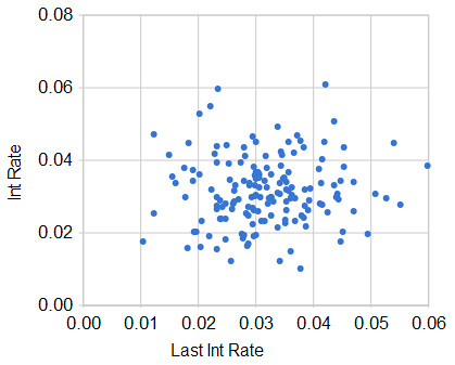 The next chart is further illustration of the randomness of defensive interceptions. It is a picture of an unyielding force in nature--regression to the mean. If interceptions are indeed random, we should expect a very strong tendency for teams to regress to the league mean from one year to the next. The year-to-year change in each team's interception rate is plotted against their previous rate. Despite some random dispersion, the trend is very clear--almost all teams with poor interception rates drastically improved the next year, and virtually all teams with very good rates significantly declined.
vs. Previous Yr Interception Rate Take the team furthest in the upper-left corner. That was the 2005 Raiders, who managed only a 1.0% interception rate. In the following season, the Raiders improved by 2.7 percentage points to a solidly above-average 3.7% rate. (The average is 3.1%.) On the other side of the chart, take the 2006 Ravens. They posted a 5.5% interception rate only to fall 3.3 percentage points to a very poor 2.2%. Very high and very low interception rates just don't persist.
 Why are interception rates so random? First, they are by nature fairly chaotic and complex events. Tipped and bobbled passes contribute to a team's total. Second, because interception stats are relatively persistent for an offense, defensive stats are driven by who the opponents happen to be. Most opponents rotate from year to year, and poor division opponents tend to improve while good ones tend to decline. Lastly, extremely good performances are usually due to a confluence of favorable factors such as injuries, player match-ups, or even weather conditions. There is no reason to expect such good fortune in consecutive years.
I'm not predicting the Chargers rate will be below average or even average. However, I am saying it is extremely likely that the Chargers will have far fewer interceptions in 2008 than they did last year. Based on recent history, by far the best bet is that they'll be pretty close to average. There's almost no possibility they'll have another year with anything close to the 5.4% rate from 2007.
Based on the historical regression trend, the Chargers would be expected to decline by 2.1 percentage points to a very average 3.3%. If the Chargers face a similar number of pass attempts as they did in 2007, they'd go from 30 interceptions to about 18.
Further, we can estimate what kind of effect this decline could have on the Chargers' record using the regression model very similar to the one discussed here. In short, all other factors being equal, a team can expect to win about 0.6 fewer games for every 1.0% decline in interception rate. In the Chargers' case, this translates to a difference of 1.3 fewer wins. The Bolts could defy gravity, but don't hold your breath.
Player IQ by Position
 Data visualization expert Ben Fry created some great graphs of each NFL position's average Wonderlic scores. Quarterbacks, centers, and offensive tackles tend to be the smartest while running backs and receivers average sub-100 IQs. The data came from this ESPN Page 2 article. Both links offer some interesting observations and comparisons. ESPN even offers you the opportunity to test yourself.
Ignore the "Read more" link. That's it.
Brett Favre Is Overrated
 The Brett Favre retirement drama is back in full swing. I don't blame him one bit for wanting to play another year, but despite the resurgent season he had in 2007, he's not the quarterback everyone thinks he is. Chances are he wouldn't have nearly as good a year as last year, especially if he goes to another team. In this article, I'll explain why.
I suddenly became a huge Brett Favre fan last year. My fantasy football draft seemed to be going well and I was excited to have Marc Bulger as my starting QB. But as the draft dragged on, I had to leave for an appointment. For my last few picks, I left instructions with a fellow team owner. One of them was to grab the top ranked remaining QB in round 15 as my backup, who turned out to be Favre. As the Rams disintegrated in the early weeks of the season, I was forced to plug in the rapidly aging Favre, who then went on to have a fantastic year and carry my team into my league's championship game.
But he didn't really have a fantastic year. His receivers did.
But getting lots of YAC is a skill you say. You say there is some special quality of a QB that allows his receivers to gain lots of YAC. It actually has far, far more to do with the receiver than the QB. No matter how we measure QB accuracy, there is scant evidence of a positive correlation between a QB's precision and his receivers' YAC.
YAC is actually a function of two primary factors: receiver ability and what type of pass is thrown. Getting YAC appears to be a persisting skill from year to year for receivers. Receivers who rack up a lot of yards one year will tend to get a lot the next. The correlation from year to year is far stronger for receivers than for QBs, an indication that the skill lies with the pass catcher, not the thrower. Additionally, YAC is determined by what kind of pass is thrown. Very difficult passes, like those "into traffic" or deep out routes (or touchdowns) tend to get little or no YAC. But easy passes like screens, flares, and "dump-offs" get very large amounts of YAC. Think of a flare or screen pass that is caught at about the line of scrimmage. The yardage would be nearly all YAC.
Ironically, the worse the quarterback, the more YAC he'll probably get. The QBs with the most YAC per pass last year included Croyle, Favre, the once-great-but-ancient Vinnie Testaverde, Brian Griese, Joey Harrington and Josh McCown--not good company.
Guys who can't throw 
I'm not saying he's awful, just that he's very overrated. He's my age, so I'm truly amazed by his durability and have respect for a competitor of his caliber. But whatever team ends up with him in 2008 will probably be very disappointed.
The table below lists 2007 QBs according to their total performance (until the final week of the season, not including receiver YAC. AY/A is "Air Yards per Attempt"--passing yards per attempt without YAC. +WP16 is the estimated wins added above average for each QB. Click on the table headers to sort.
| Rank | Quarterback | QBRat | Att | Yds | Int | Rush | Yds | Sk Yds | Fum | AY/A | %YAC | +WP16 |
| 1 | Brady | 119.7 | 503 | 4235 | 6 | 29 | 91 | 107 | 4 | 4.9 | 42 | 2.48 |
| 2 | Garrard | 101.6 | 307 | 2310 | 2 | 45 | 166 | 91 | 3 | 4.8 | 37 | 2.21 |
| 3 | Manning P | 95.2 | 464 | 3634 | 14 | 19 | -4 | 122 | 5 | 4.9 | 37 | 1.29 |
| 4 | Anderson | 85.8 | 459 | 3384 | 14 | 30 | 64 | 100 | 5 | 4.5 | 38 | 0.95 |
| 5 | Romo | 101.0 | 462 | 3868 | 17 | 25 | 116 | 166 | 9 | 4.9 | 41 | 0.89 |
| 6 | Schaub | 87.2 | 289 | 2241 | 9 | 17 | 52 | 126 | 7 | 5.0 | 36 | 0.87 |
| 7 | Roethlisberger | 104.1 | 404 | 3154 | 11 | 35 | 204 | 347 | 9 | 5.2 | 34 | 0.86 |
| 8 | Cutler | 90.8 | 398 | 3096 | 12 | 41 | 163 | 119 | 8 | 4.3 | 44 | 0.46 |
| 9 | Garcia | 93.6 | 307 | 2244 | 4 | 34 | 116 | 98 | 3 | 3.7 | 50 | 0.44 |
| 10 | Palmer | 86.2 | 522 | 3700 | 17 | 22 | 11 | 119 | 5 | 4.3 | 40 | 0.36 |
| 11 | Hasselbeck | 92.0 | 510 | 3620 | 10 | 35 | 68 | 183 | 8 | 4.0 | 44 | 0.17 |
| 12 | Brees | 92.1 | 550 | 3819 | 15 | 22 | 53 | 89 | 7 | 3.8 | 45 | 0.11 |
| 13 | Favre | 97.7 | 492 | 3905 | 13 | 25 | -9 | 89 | 8 | 3.8 | 52 | -0.16 |
| 14 | Warner | 87.6 | 360 | 2748 | 15 | 13 | -4 | 140 | 11 | 4.7 | 38 | -0.22 |
| 15 | Kitna | 84.6 | 497 | 3707 | 17 | 21 | 55 | 304 | 15 | 4.7 | 37 | -0.26 |
| 16 | McNabb | 86.8 | 397 | 2716 | 6 | 43 | 199 | 192 | 7 | 3.4 | 50 | -0.33 |
| 17 | Campbell | 77.6 | 417 | 2700 | 11 | 36 | 185 | 110 | 13 | 3.6 | 44 | -0.44 |
| 18 | Jackson | 69.6 | 222 | 1516 | 10 | 42 | 180 | 47 | 3 | 3.6 | 47 | -0.58 |
| 19 | Pennington | 85.8 | 228 | 1501 | 7 | 18 | 27 | 142 | 3 | 4.1 | 38 | -0.61 |
| 20 | Boller | 75.2 | 275 | 1743 | 10 | 19 | 89 | 159 | 5 | 4.0 | 37 | -0.74 |
| 21 | Young | 70.1 | 342 | 2223 | 16 | 82 | 375 | 132 | 7 | 3.5 | 46 | -0.92 |
| 22 | Edwards | 75.6 | 213 | 1336 | 5 | 9 | 25 | 71 | 2 | 3.1 | 51 | -0.94 |
| 23 | Bulger | 71.4 | 353 | 2216 | 13 | 9 | 13 | 248 | 6 | 4.1 | 35 | -1.11 |
| 24 | Manning E | 72.6 | 482 | 2974 | 17 | 24 | 56 | 186 | 7 | 3.5 | 43 | -1.11 |
| 25 | Losman | 76.9 | 175 | 1204 | 6 | 20 | 110 | 103 | 4 | 3.4 | 50 | -1.21 |
| 26 | Rivers | 80.0 | 412 | 2828 | 15 | 26 | 31 | 153 | 10 | 3.7 | 46 | -1.22 |
| 27 | Culpepper | 78.0 | 186 | 1331 | 5 | 20 | 40 | 130 | 8 | 4.0 | 44 | -1.24 |
| 28 | Harrington | 77.2 | 348 | 2215 | 8 | 14 | 33 | 192 | 0 | 3.0 | 52 | -1.26 |
| 29 | Smith | 57.2 | 193 | 914 | 4 | 13 | 89 | 121 | 6 | 3.1 | 35 | -1.43 |
| 30 | Lemon | 69.9 | 247 | 1479 | 6 | 25 | 86 | 120 | 6 | 3.0 | 50 | -1.52 |
| 31 | Clemens | 59.0 | 225 | 1414 | 10 | 19 | 93 | 125 | 4 | 3.4 | 46 | -1.80 |
| 32 | McNair | 73.9 | 205 | 1113 | 4 | 10 | 32 | 85 | 8 | 2.8 | 49 | -2.02 |
| 33 | Huard | 72.6 | 296 | 1952 | 13 | 9 | -1 | 204 | 4 | 3.6 | 45 | -2.03 |
| 34 | Grossman | 66.4 | 225 | 1411 | 7 | 14 | 27 | 198 | 6 | 3.5 | 44 | -2.03 |
| 35 | Griese | 75.6 | 262 | 1803 | 12 | 13 | 28 | 114 | 6 | 3.3 | 52 | -2.22 |
| 36 | Testaverde | 65.8 | 172 | 952 | 6 | 8 | 23 | 46 | 3 | 2.6 | 52 | -2.24 |
| 37 | Frerotte | 62.0 | 162 | 1010 | 11 | 6 | 3 | 59 | 3 | 3.9 | 38 | -2.34 |
| 38 | McCown | 68.6 | 182 | 1105 | 11 | 29 | 143 | 78 | 10 | 3.0 | 51 | -3.14 |
| 39 | Croyle | 71.7 | 169 | 963 | 5 | 5 | 16 | 72 | 4 | 1.8 | 68 | -3.57 |
| 40 | Dilfer | 55.1 | 219 | 1166 | 12 | 10 | 25 | 182 | 8 | 3.0 | 43 | -3.87 |
| Rank | Name | QBRat | Att | Yds | Int | Rush | Yds | Sk Yds | Fum | AY/A | %YAC | +WP16 |
Jared Allen and Sack Rate
 The biggest transaction this off-season may have been the Jared Allen trade from Kansas City to Minnesota. Allen led the league in sacks last year with 15.5. He'll be going to a Viking defensive line that was impenetrable against the run but featured an average pass rush. The Vikings defense was so good against the run, opponents passed nearly 70% of the time compared to a league average of about 55%. Allen's ability as a pass rusher could have a very large impact. We know the Vikings pass rush will probably improve, but by how much? And how will the improvement affect the Vikes' bottom line?
Importance of Sacks
First, let's look at the general importance of sacks in terms of team wins. Normally when I model team wins, I combine sack stats with passing stats to calculate net passing yards. Along with turnover rates, running efficiency, and penalty rates, net passing efficiency is used in a regression to estimate total season wins for any given team. This method is useful for estimating the overall importance of the passing game compared to other aspects of football. But in this case, we want to specifically know the effect sacks have on total team wins.
By using basic yards per attempt (YPA) and sack rate instead of net passing efficiency, we can isolate the effect sacks have on winning. Using sack rate (sacks per drop back) instead of total sacks is useful for two reasons. First, it is far less susceptible to problems caused by the direction of causation. That is, defenses that face lots of passes would tend to have higher sack totals because they have more opportunities. Secondly, it allows us to compare teams and players that faced vastly different numbers of pass attempts (such as the Chiefs and Vikings).
Jared Allen's Potential Effect Allen's 15.5 sacks were remarkable because he played in only 14 of 16 games last season. He also played on a 5-11 team that more often than not faced offenses with safe leads more interested in running out the clock than passing. His sack rate was an amazing 3.8%. That's as high as the entire entire Bengals' defense. Had he played in all 17 games and faced the very high number of passes the Vikings defense faced, Allen would have over 26 sacks! But it's unlikely the Vikings' opponents will pass nearly as often in 2008, especially with Allen leading an improved pass rush. If they face the average number of drop-backs, Allen would have about 20 sacks, still a near-record-high amount.
In estimating the number of added sacks Jared Allen could bring to the Vikings, we can't just add 20 to their previous total of 36. The Vikings defense already had 9.5 sacks from the right DE position last year, 5 from Ray Edwards and 4.5 from Brian Robison. A reasonable estimate would be that Allen could add a net of 10 additional sacks, taking them from an exactly average 36 sacks to a solidly above-average 46. This assumes he performs nearly as well as last year and he remains healthy--both fairly big assumptions.
Note that the additional sacks Allen may bring need not be his sacks. By chasing a QB out of the pocket or by occupying multiple pass blockers Allen could enable teammates to get the sack, but the credit would still belong to him.
Sack Rate's Contribution to Winning
Based on a regression of team win totals using sack rates, running and passing efficiencies, turnover rates, and penalty rates, sack rates are fairly important. For every standard deviation improvement in sack rate, a team can expect about an additional half win. That's comparable in importance to offensive running efficiency. The table below lists other important stats in comparison to sack rate and how they tend to impact team win totals.
Effect on Wins per Standard DeviationStatistic Wins per SD O Pass Efficiency 1.15 D Pass Efficiency 0.97 D Sack Rate 0.47 O Run Efficiency 0.43 D Run Efficiency 0.25
Stated differently, for every percentage point increase in sack rate, a team can expect an extra 0.36 wins. Jared Allen's additional 10 sacks would improve the Vikings' sack rate from 5.0% to 6.4%. That additional 1.4% roughly translates into 0.50 additional wins for Minnesota.
Sacks correlate with other defensive stats, which complicates the analysis. Sack statistics are representative of a defense's overall pass rush. There are hurries and QB hits that are interrelated with other stats such as defensive passing efficiency, interceptions, and fumble rate. (I'll have to make one more assumption--that a pass rush causes the effect on passing efficiency, fumbles, and interceptions instead of the other way around. I realize this is not absolutely correct. A good secondary can cause the QB to hold the ball longer, for example. But it appears to me that the direction of causation primarily begins with the pass rush.) The fact that sacks correlate with defensive passing efficiency, interceptions, and fumbles means that the benefit of adding a solid pass rusher is stronger than it first appears. Unfortunately, it also means the regression model is less than perfect. Ideally all of the independent variables in a regression are independent of each other as well as independent of the dependent variable. (This is why my normal model does not break out sacks and uses net pass efficiency instead.) However, no model is ever perfect, and I could only hope for a solid but rough 'order-of-magnitude' estimate anyway.
I estimated the effect of sack rate on defensive passing efficiency, interception rates, and fumble rates. I won't bore you any further with regression results, but the correlations were:Statistic Correlation with Sack Rate D Pass Efficiency 0.21 D Int Rate 0.17 Fumble Rate 0.43
In short, the cumulative effect of sacks on these other stats contributes to an additional 0.41 wins. In total the Vikings could expect about 0.9 additional wins from an extra 10 sacks. Realistically, this estimate should be taken as very rough, but it does provide an idea of the magnitude of impact a premier pass rusher could provide his team.
Baseball Experts: Dumber than Monkeys
 I’ve noted before just how bad expert predictions of NFL season outcomes usually are. It appears to be the same in baseball too. This site tracked and graded 42 expert predictions of which teams would be in first place in each division. Although we’re only just past halfway through the baseball season (the rankings are as of July 1st), 90 games into a season is not too soon to check in on how the experts are faring as a group. There’s little reason to expect much improvement in them between now and September. This article will take a look at just how well the experts do as a group. (Does the title kind of give it away?)
The grading system assigns 12 points to each expert for predicting the current division leader, and then assigns a proportional amount for trailing teams based on how many games out of first they are. For example, someone who predicted the Cubs would be leading the NL Central, he’d receive 12 points. If he had picked the 2nd place Cardinals to win the division, he’d get 10. But if he had picked the cellar-dwelling Reds, he’d get only 1 point.
Of the 42 experts tracked, the two best prognosticators each scored 64 points under the system, which seems pretty good because picking all 6 division leaders would add up to 72 points. But with so many experts, a few are bound to end up with very good scores just by luck alone. Do these experts have any real predictive ability, or is it just luck?
If there was a room full of monkeys (or Sports Center analysts) making predictions purely at random, they’d get an average of 39.5 points according to the scoring rules. The experts’ actual average score was 48.6. Things are looking pretty good for the experts so far.
But the experts had a huge advantage over the monkeys. They can read. Using last season’s standings as a basis for this season’s predictions would score 59 points. How does the experts’ average of 48.6 look now?
Below is the distribution of the experts’ actual scores. For example, 3 experts scored up to 33 points, and 5 experts scored between 34 and 38 points, and so on. I’ve also drawn a normal distribution based on the experts’ actual scores for comparison.
But as I noted above, last year’s standings would be the most logical starting point for making this season’s predictions. Since the experts had the benefit of this prior knowledge, even if they had absolutely no analytic or predictive ability, the distribution of scores should be bunched around the 59-point baseline of last year’s standings. Some experts would score higher while others would score lower, due to either luck or true analytic ability. And if they had any real predictive ability, they should usually score at least that well.
The next graph shows the actual distribution of the experts compared the distribution of how it should look by using the information from the prior season. (It would actually be slightly non-normal and asymmetrical because of being bounded at a 72-point maximum.) Remember, this is still monkeys guessing randomly, but this time their starting point is the 59 points based on last season. How do the experts compare to monkeys who can read last September’s standings?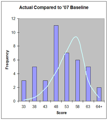
It turns out the experts aren’t even close to the sports-page-reading monkeys. The distribution of prediction scores is about halfway between last season’s baseline and totally random.
My point is that as we approach football’s silly season of predictions, don’t believe anything you read or hear. Don’t put much stock in a favorable prediction for your team, and don’t panic at an unfavorable one.
Tangentially, I’ve learned something about predictions from the traffic of my site. If I do an analysis that turns out to be favorable for a team’s outlook, such as the Jared Allen article, my site gets linked around the Vikings fan community (which I appreciate—don’t get me wrong). And if I do a negative article, such as the one about Favre, people are interested, but there’s not as much excitement. So if I had ads on my site, I’d be temped to heavily skew my analysis positively, giving every fan a reason for hope. I’d probably go around the league, targeting certain markets with fancy-schmancy math about how awesome their team is going to be. Except for you, Pittsburgh fans. You guys are going to stink this year. Besides, you don't understand math. (That's another technique--create controversy.) My traffic would explode, and I’d make a little money. I get the feeling much of the national sports media probably does just this sort of thing. Everyone is selling hope I suppose, even to poor, stupid Steeler fans.
Hat tip: King Kaufman.
Follow-Up on Game Theory and The Passing Premium
 The strategy of play selection on both offense and defense is one of the most compelling aspects of football. Most other sports don't feature such a strategic battle on every play. The balance between running and passing has long been at the center of football strategy debate. Research on the run/pass balance has mostly focused on the "passing premium"--the apparent difference in average expected yards yielded by a pass compared to a run.
Here is a great discussion of the importance of game theory in understanding run/pass balance at Tom Tango's sabermetrics site. "MGL's" comments are particularly insightful. In this post, I'll try to summarize some of the discussion's main points (in bold) and offer my own thoughts (in normal type).
1. It's true that according to game theory, when a game is in equilibrium between two strategy options (like run and pass), the expected outcomes of both strategies will be of equal value. Recent research papers use expected yards (sometimes accounting for risk premiums) as the measure of value. They expect average yards gained by running and passing to be equal at the optimum proportion of each strategy. But the assumption that yards = value in football is mistaken. Often, an offense faces 3rd and 8, and 7 yards just won't help any more than 3 yards. Also, time has to play a factor. It may be better for a winning team to trade yards for time off the clock. The entire analysis hinges on a valid utility function for football.
2. It would be extremely difficult to actually chart the utility matrix and solve the equilibrium between running and passing. This is undoubtedly true. We would need to have good data for when a defense is 100% sure that the play will be a pass and for when a defense is certain the play will be a run. There are some situations which may be close enough to "certain pass" or "certain run" to shed some light. We would need such data to pin down the normal form of the game, i.e. the payoff matrix. This assumes we have a valid utility function.
3. The '10 yards in 4 downs' rule severely complicates the analysis. This is true, as the utility of 3 yards is very different on 3rd and 1 than it is on 3rd and 10. However, we can isolate the analysis at specific down and distance situations. We could start with 1st and 10s as commenter Chris suggested. (He also suggested charting 3rd downs as binary--success or failure.) I'd also want to limit it to ordinary game situations such as between the 20-yard-lines and prior to the 4th quarter.
4. There is a difference between the "optimum" strategy mix and the "equilibrium" strategy. In game theory, the Nash equilibrium (NE) is the strategy mix of both opponents at which neither would benefit from unilaterally changing his own mix. Let's say on 1st and 10 in ordinary situations, the NE solution is for the offense to play 60% run/40% pass and for the defense to play 60% run D/40% pass D. The offense can guarantee itself a minimum average payoff by playing the 60/40 NE, and if the defense played its NE mix, the "equilibrium" mix would indeed be "optimum" for both teams. Neither team would benefit from altering its mix.
However, if the defense failed to play the correct mix, and played 50/50 for instance, equilibrium and optimum are no longer the same. The offense can continue to guarantee itself a minimum average payoff by playing the 60/40 NE mix, but it could get more by taking advantage of the defense's mistake. The offense's optimum mix might now be 70/30 or so. Because the defense is overplaying pass D, the offense should run more often. (In theory, the offense should run 100% of the time to optimize. But in repeated iterations, this would too obvious and even the most oblivious defense would adjust.)
There are several other insightful comments there. The baseball guys are a little further along thinking about these kinds of things. For example, there is tremendous similarity between the run/pass strategy game between offense and defense, and the fastball/curve game between pitcher and batter.
I realize the game theory aspect of the run/pass balance question is very obvious in a way. Even the dimmist TV commentators talk about the run setting up the pass. But I think it's useful to think about the topic in a more formal way, and let the math inform us.