
 Before Michael Vick's run-in with the law, he was widely considered an exciting and elusive quarterback with below-average throwing ability. Usually, his poor completion percentage is cited as evidence of his lackluster passing ability. It seems that reputation is still with him. Case in point is this excerpt from Peter King's most recent post:
Well, as a quarterback, Vick was decidedly mediocre in his four full seasons starting for the Falcons. His completion percentages when he started at least 15 games -- 54.9, 56.4, 55.3 and 52.6 -- were poor; he had 36 fumbles and 38 interceptions in his last 46 starts.
One thing is certain--Vick is (or was) an unconventional QB. He was a breakaway runner without peer, and the normal rules of quarterbacking don't apply. The vast majority of Vick's 529 career runs were scrambles on pass plays. When a conventional QB progresses through his reads, he looks at WR#1, WR#2, TE, and then dumps off to a RB. But Vick, on the other hand, doesn't bother with the dump off. He is the dump off.
Most of Vick's 52 running yards per game can really be credited as passing yards. They were yards gained on pass plays in passing situations. He averaged 7.1 yards per run. Compare that to the NFL's 5.0 average net passing yards per attempt and 4.1 rushing yards per attempt. And remember, there is never a risk of interception if he tucks the ball and runs. If you factor in his sacks into his rushing average, it becomes 5.1 net yards per run, which is still good. But if we do that, it would make his net passing yards per attempt much higher. After all, we can only count his sack yards against him once. Otherwise, it's double jeopardy.
So Vick's pass completion stats aren't padded by lots of rinky-dinky dump offs. David Carr actually led the NFL in completion percentage in 2006 with a gaudy 68.3%, only to lose his job the following off-season (to Vick's backup nonetheless).
To get an idea of how deep Vick was throwing compared to his league counterparts, we can look at yards per completion. In 2006, the most recent year Vick played, the league's other top 30 QBs averaged 11.4 yards per completion, while Vick averaged 12.1.
Vick's receiver corps in Atlanta was never known as particularly talented. If we remove receiver YAC from the equation, the numbers are even more favorable for Vick. His Air Yards, the yards a complete pass travels in the air forward of the line of scrimmage, is impressive. The top 30 other QBs in 2006 averaged 6.3 Air Yds per completion, while Vick averaged 7.7.
Yes, his interception and fumble rates are higher than you'd like, but those too should be considered in the context of the depth of his throws and the frequency with which he runs. So although Vick's passing stats, especially completion percentage, appear sub-par, that should be expected, and they are somewhat offset by greater gains for each completion. I'm not claiming he's great, or even above average, just better than his conventional stats suggest.
Michael Vick Was a Better QB Than You Think
Are NFL Coaches Too Timid?
 Risk is at the heart of football strategy. Aggressive, risky gameplans should result in boom-or-bust high-variance outcomes, sometimes scoring lots of points but sometimes scoring very few. Conservative gameplans result in relatively consistent low-variance outcomes. Teams would more likely score close to their average score.
In this post, I’ll look at what high and low variance strategies would look like in terms of point totals and how they affect each team’s chances of winning. I’ll also compare the theoretical strategies to the actual distributions in the NFL. We'll see why NFL coaches should be more aggressive when they're the underdog.
High Variance Strategy in Basketball
Some time ago, I came across an article posted by basketball researcher Dean Oliver that analyzed high and low variance strategies for the NBA. Oliver calculated the win probability of each opponent according to the mean and standard deviation (SD) of each team’s scoring tendencies. SD represents the degree of variance. The more aggressive and riskier the strategy, the higher the SD will be. For example, a basketball team that shoots lots of 3-pointers would have a high variance.
The key to accurately modeling basketball is realizing that each team’s score is correlated with that of its opponent. The pace of a basketball game ties each team’s score together, and there is a high level of covariance. When one team scores a high number of points, the other team will tend to score more too. Game scores are interdependent.
In Football
Recently the Smart Football blog illustrated the advantage of high variance strategies for underdogs. A high variance strategy increases an underdog’s chances of winning but comes with the cost of also increasing its chances of being blown out.
In the NFL as a whole, visiting teams average about 19 points with a SD of 10 points while home teams average about 23 points with a SD of 10 points. But unlike basketball, football opponent scores are negatively correlated. This makes intuitive sense because the better one team does, the worse the other should do. If one team gets lots of first downs and doesn’t commit turnovers, its opponent will usually start drives with poor field position, and vice versa. The covariance between NFL opponent scores is -1.9 points-squared.
If NFL scores were normally distributed, this is what the typical score distribution would look like. The visitor scores are in red and the home scores are in blue.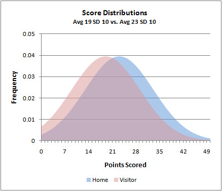
We can calculate each team's chances of winning by summing all the probabilities with these distributions and factor in the covariance using Dean Oliver’s method. This estimates that the home team wins 56.5% of the time, which happens to be exactly the NFL actual home field advantage.
Disclaimer
There’s one problem. NFL scores are not normally distributed, primarily due to its unique scoring, which typically comes in chunks of 3 or 7. Here is what the actual distribution of scores looks like.
The good news is, if we group the scores into bins of 7 points, we get a quasi-normal distribution. (Technically, it may be more of a gamma or Poisson distribution.) I’m going to stick with normal distributions to simplify the math and to better illustrate the concepts I want to convey.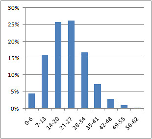
Demonstration
Here’s why underdogs should play aggressive and risky gameplans. Take an example where one team is a 7-point favorite over its underdog opponent. Say the favorite would average 24 points and the underdog would average 17 points. With a SD of 10 points for each team, the underdog upsets the favorite 31.5% of the time. The favorite’s scoring distribution is blue and the underdog’s is red.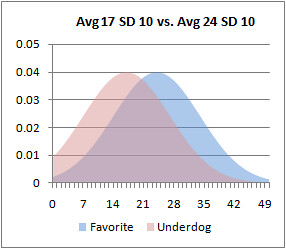
But if the underdog plays a more aggressive high-variance strategy, increasing its SD to 15 points, it would upset the favorite 35.3% of the time.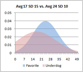
Note that I haven’t increased the underdog’s average score in any way, just its variance. The increase in its chance of winning results due to more of its probability mass moving to the right of the favorite’s mean score of 24. In fact, the higher the variance, the wider the probability mass will be spread. Consequently, more mass will be to right side of the favorite’s average score. But more mass will also be to the left, meaning there is a higher risk of an embarrassing blowout.
Even if employing a high-variance strategy is non-optimum, it can still help an underdog. In other words, even if an aggressive gameplan results in an overall reduction in average points scored, it often still results in a better chance of winning.
The next graph plots the scoring distributions of just such a scenario. Like before, the favorite’s average score is 24 with a SD of 10. But this time the underdog’s average is reduced from 17 to 16. The increase in variance still results in a slightly better chance of winning despite its overall reduction in average points scored. In this case, it's 33.2% for the underdog.
What about the favorite? Should it increase its variance in response to an aggressive underdog? No. Ideally it should play as consistently as possible. The lower the variance the better for the favorite. The next example shows a favorite playing a low-variance game with an average of 24 points and a SD of 5 points. The underdog is playing conventionally with a 17 point average and 10 point SD. The result is an increase in the favorite’s chances of winning from 69.5% in the original example to 73.0%.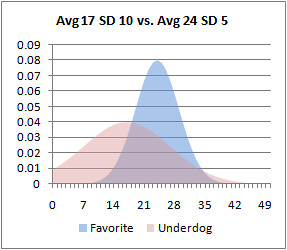
And if the underdog plays an aggressive high-variance game, the low-variance strategy is still better for the favorite. In this case the favorite still improves its chances of winning from 64.7% to 67.8%.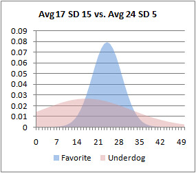
In Practice
So what does any of this mean in the real world? Simply put, to win more often underdogs should employ a high-variance strategy from the beginning of the game. It shouldn’t wait until the 4th quarter and become desperate. Go for it on 4th and short, run trick plays, throw deep, and blitz more often. Roll the dice from the get-go.
The real question is, what is the optimum level of risk? I’m not sure, but I do know NFL coaches are operating far from it.
Looking at games from the ’02 through ’06 seasons (a total of 1280), underdogs do not increase their variance. For example, for games in which the point spread is between 6 and 7.5 points, the underdog’s SD is 9.8 points, slightly less than the overall league average. Ideally, it should be higher. The favorite’s SD is 10.4 points when ideally it should be lower.
The table below lists the SDs of points scored for the favorite and underdog according to the most common point spreads.
| Spread | Favorite SD | Underdog SD |
| 0 - 1.5 | 9.6 | 10.5 |
| 2 - 3.5 | 9.8 | 9.4 |
| 6 - 7.5 | 10.4 | 9.8 |
| 10 - 11.5 | 10.5 | 8.7 |
If anything, there appears to be slight trends in the exactly wrong directions. The bigger the spread, the smaller the underdog’s variance and the bigger the favorite’s variance. It appears underdogs may get less aggressive while favorites may get more aggressive.
Conclusions
This is more evidence coaches do not coach to maximize their team’s chances of winning. My theory is coaches are delaying elimination until the latest point in the game—that is, trying to “stay in the game” for as long as possible. Underdog coaches minimize risk all game long hoping for a miracle along the way. They seem to be reducing the chances of being blown out, but this is not consistent with giving their team the best chance to win.
But if you think about it, this kind of approach might be good for the NFL as a whole. It keeps games entertaining as long as possible, and keeps viewers tuned in.
Coaches of favored teams could be accused of the same crime. They might be playing with too much variance. But there is certainly a limit to just how consistent a team can be, no matter how hard it tries. There will always be random variation in team performance. I suspect a SD of 10 points may be near that limit, and that coaches of both favorites and underdogs simply play the least risky game they can consistent with accepted conventions.
Thoughts on the Apparent Unimportance of Run Defense
 John Morgan of the Seahawks blog Fieldgulls.com asked me recently about why run defense appears relatively less important in terms of winning than do other facets of the game. John writes:
You state defensive rushing yards per attempt allowed is the least important component to winning, but I wonder if that factors in game situation. Losing teams are likely to reduce their yards per attempt allowed when winning teams are running out the clock.
John makes a good point, and indeed the team-stat regression model I used when I made that conclusion did not take game situation into account. John goes on to point out that teams that are already behind may face a large number of predictable run-out-the-clock runs, which would make their run defense appear better. Plus, the game theory aspects of running and passing should enable a good run defense to make stopping the pass easier.
I think this is an interesting point, and I soon should be able to test how much late-game runs affect a team’s overall defensive efficiency after some improvements to my play-by-play database. A preliminary look indicates it probably doesn’t make much of a difference. Still, I think John raises good points about the game theory aspect and predictability.
In theory, good a run defense should make a pass defense better. And the stats suggest it does. The correlation between defensive running efficiency and passing efficiency is 0.20. Some of that correlation has to do with the fact that superior defensive athletes are superior against both the run and the pass. But some of it should also be due to the game theory aspect.
(In comparison, offensive running and passing efficiency correlate at 0.13. I think the difference is that there is a lot more variance in offensive passing than in other facets due to the focus on a single player’s ability. The quarterback’s contribution is so critical to passing in ways that aren’t applicable to the other aspects.)
According to game theory principals, defensive running and passing would only be equally important if offenses and defenses were operating at the game equilibrium point-- that is, they’re playing the optimum mix of passing and running. But I think they might not be.
My theory is that this may be why run defense appears so unimportant. Say teams are not operating at the game equilibrium, and passing is, on balance, a more lucrative strategy than running. In other words, there really is a considerable passing premium where the payoff for a pass is generally higher than a run, all things considered.
Having a good run defense would therefore be somewhat self-defeating. Take the 2007 Vikings defense that gave up only 3.1 yards per run (good) but 7.0 yards per pass (bad). Facing such a solid run defense, a good offensive coordinator is forced to pass more…which would be a far more effective thing to do in the first place, especially against a relatively weak pass defense. A team like the 2007 Vikings would essentially be forcing their opponent to unwittingly play a more efficient and effective strategy, all the while exploiting their own weakness.
Should Rookie QBs Start?
 Wages of Wins author and loyal Detroit Lions fan Dave Berri recently asked me about research on whether rookie quarterbacks are better off standing on the sideline all season. One of the big questions in Detroit this year will certainly be whether overall number one pick Matthew Stafford should start at QB. The central issue is whether starting a rookie QB somehow harms his long-term development. Does a year holding a clipboard allow rookies to adapt to the NFL and boost their prospects for a successful career?
Names like Boller, Harrington, Couch, Shuler, and Carr underscore the danger of starting rookie passers. But there are also names such as Manning, Roethlisberger, Marino, Elway, and Aikman that indicate that starting as a rookie may not be so damaging to a QB's development.
This is a question I get often but haven’t looked into it because of complications associated with the issue. First, there aren’t that many top QBs to analyze—the sample size is fairly small. Any inference we make needs to keep in mind the small sample. Second, there is a problem of bias in the data. The better QBs would be the ones to earn starting jobs their rookie year, and would also likely tend to be the ones to enjoy successful careers.
The trick would be to properly account for underlying QB potential, which would be quite a trick. If we knew that, that’s all we’d ever really need to know about a QB. There's no perfect way to measure that, but in the end, I think the most reasonable variable to indicate potential is overall draft pick number. It’s something that is established prior to any decision to start or not as a rookie. Also, although it is often an unreliable predictor of career performance for individual QBs, it correlates very well for QBs as a group. In other words, the number one QB might not pan out or even be better than the second QB taken in any particular draft year. But as a whole, the top picks reliably tend to outperform subsequent picks.
Data
I looked at first and second round QBs drafted between 1980 and 2004. I chose 1980 because it is roughly the dawn of the modern NFL passing rules. I chose 2004 to allow at least four years to asses each QB’s performance. Data are from Pro-Football-Reference.com. To measure career success, I used Adjusted Yards per Attempt (Adj YPA). This is passing yards minus 45 yards for every interception, per pass attempt. For QBs with very low pass attempts and spurious Adj YPA stats, I replaced their actual Adj YPA with 3.0 YPA, generally the floor for QBs with a reasonable sample size of attempts. (There is no reason to expect 1989 Chief’s 2nd-round pick Mike Elkins to lose 20 yards for every pass based on only 2 attempts.)
Methodology
The first step is to account for potential using overall draft pick number. The graph below plots career Adj YPA by pick number. The scatterplot is pretty random for any individual QB, but as a whole there is a predictable trend. Top draft picks tend to end up as NFL top passers. I estimated the expected Adj YPA based on pick number. A QB from the top of the first round would be expected to average 5.0 Adj YPA, while a QB from the bottom of the second round would be expected to average 4.1 Adj YPA.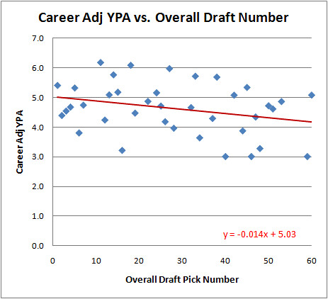
We can see a clear trend. Unsurprisingly, top picks would be expected to end up with better career passing stats than later picks. A linear regression estimates what the baseline expectation should be for each slot in the draft.
Next I calculated the 'Adj YPA above expected' for each QB. Now we can compare QBs who started their first year to those that didn’t, while holding “potential” equal.
But how do we define “started their first year?” How many starts qualifies--4, 5, 11? I don’t know, so let’s start by looking at the whole picture.
Results
We can use that baseline to compare each QB's career Adj YPA. Some QBs did better than expected given their draft slots and some did worse. We can now test if there is a connection between better than expected performance and the number of rookie year starts.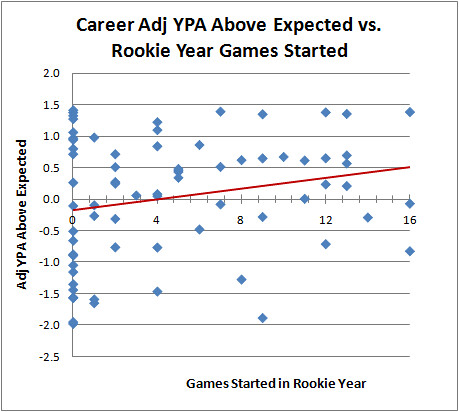
As it turns out, it appears that QBs with more rookie starts tend to enjoy greater career success, even accounting for draft order.
Some of you might have noticed that what I've really done here is a crude multivariate regression. Holding for draft order, I estimated the effect of games started. What if we just do the regression directly?
As expected we get a small negative effect with draft order. (The higher the pick number, the worse the expected stats.) The Games Started variable is positive and significant at p=0.03. The model as a whole has an r-squared of 0.15--small in absolute terms, but considerable given the highly random individual variance in QB careers.
But this is only one way of looking at whether a QB was a starter or not. What if we draw a line at say, 5 rookies starts--below 5 starts he's not a rookie starter and above it he is. The group of QBs with 5 or less starts averages -0.01 Adj YPA above expected, and the group with 6 or more starts averages +0.3 Adj YPA above expected. If we define it at zero starts, those with no rookie starts averaged -0.03 Adj YPA above expected, while those with at least one start averaged +0.02 starts above expected. In fact, no matter where I chose the endpoints of the groups, from 3 to 13 starts, the group with more starts outperforms the group with fewer starts by about 0.4 Adj YPA.
Conclusion
Does this mean teams should rush their rookies out to face the onslaught of NFL defenses to somehow make them better? I really doubt it. If I had to bet, I'd say that we simply haven't fully accounted for QB "potential" using draft order alone. I think the better QBs, those with the best chances of career success, often gain and maintain starting positions earlier.
But at the very least, we can say this: Given this analysis, there is no reason for a coach to arbitrarily keep a rookie QB on the bench. He should start his best QB, rookie or not, and not worry about incubating him under a ballcap on the sidelines. In the end, it should be the coach's qualitative judgment on the readiness of the player.
Here are the QBs and their stats I used for this article. (It's interesting just to see who the QBs are who exceeded expectations. There are some surprising names--Pennington and Batch at the top, for example. And Is Eli Manning really worse than David Carr? Wow.) You can sort the table by clicking on the column headers.Year Rnd Pick Name Team Adj YPA Exp Adj YPA Yr1 GS AdjYPA Abv Exp 2001 2 32 Drew Brees ![]()
6.0 4.6 0 1.4 1981 2 33 Neil Lomax ![]()
5.9 4.6 7 1.4 1998 1 1 Peyton Manning ![]()
6.4 5.0 16 1.4 1998 2 60 Charlie Batch ![]()
5.5 4.1 12 1.4 2004 1 4 Philip Rivers ![]()
6.4 5.0 0 1.4 2004 1 11 Ben Roethlisberger ![]()
6.2 4.9 13 1.3 1983 1 27 Dan Marino ![]()
6.0 4.6 9 1.3 2000 1 18 Chad Pennington ![]()
6.1 4.8 0 1.3 1999 1 11 Daunte Culpepper ![]()
6.1 4.9 0 1.3 1984 2 38 Boomer Esiason ![]()
5.7 4.5 4 1.2 1985 2 37 Randall Cunningham ![]()
5.6 4.5 4 1.1 1983 1 24 Ken O'Brien ![]()
5.7 4.7 0 1.1 1995 2 45 Todd Collins ![]()
5.3 4.4 1 1.0 1991 2 33 Brett Favre ![]()
5.5 4.6 0 1.0 1983 1 14 Jim Kelly ![]()
5.8 4.8 0 0.9 1999 1 2 Donovan McNabb ![]()
5.9 5.0 6 0.9 1983 1 15 Tony Eason ![]()
5.7 4.8 4 0.8 2003 1 1 Carson Palmer ![]()
5.8 5.0 0 0.8 1987 1 26 Jim Harbaugh ![]()
5.4 4.7 0 0.7 1995 1 3 Steve McNair ![]()
5.7 5.0 2 0.7 1996 2 42 Tony Banks ![]()
5.1 4.4 13 0.7 1983 1 1 John Elway ![]()
5.7 5.0 10 0.7 1990 1 1 Jeff George ![]()
5.7 5.0 12 0.6 1997 2 42 Jake Plummer ![]()
5.1 4.4 9 0.6 2001 2 53 Quincy Carter ![]()
4.9 4.3 8 0.6 1989 1 1 Troy Aikman ![]()
5.6 5.0 11 0.6 2003 1 7 Byron Leftwich ![]()
5.5 4.9 13 0.6 1982 1 5 Jim McMahon ![]()
5.5 5.0 7 0.5 1995 2 60 Kordell Stewart ![]()
4.7 4.1 2 0.5 1986 1 3 Jim Everett ![]()
5.5 5.0 5 0.5 2002 1 32 Patrick Ramsey ![]()
5.0 4.6 5 0.4 1999 2 50 Shaun King ![]()
4.7 4.3 5 0.4 1989 2 51 Billy Joe Tolliver ![]()
4.6 4.3 5 0.3 2001 1 1 Michael Vick ![]()
5.3 5.0 2 0.3 2004 1 22 J.P. Losman ![]()
5.0 4.7 0 0.3 1987 1 13 Chris Miller ![]()
5.1 4.9 2 0.2 1993 1 1 Drew Bledsoe ![]()
5.3 5.0 12 0.2 1995 1 5 Kerry Collins ![]()
5.2 5.0 13 0.2 1987 1 1 Vinny Testaverde ![]()
5.1 5.0 4 0.1 2003 1 22 Rex Grossman ![]()
4.8 4.7 3 0.1 1992 1 25 Tommy Maddox ![]()
4.7 4.7 4 0.0 1986 2 47 Jack Trudeau ![]()
4.3 4.3 11 0.0 2002 1 1 David Carr ![]()
5.0 5.0 16 -0.1 2004 1 1 Eli Manning ![]()
4.9 5.0 7 -0.1 1991 1 24 Todd Marinovich ![]()
4.6 4.7 1 -0.1 1980 1 15 Marc Wilson ![]()
4.7 4.8 0 -0.1 1990 1 7 Andre Ware ![]()
4.7 4.9 1 -0.3 2003 1 19 Kyle Boller ![]()
4.5 4.8 9 -0.3 1999 1 1 Tim Couch ![]()
4.7 5.0 14 -0.3 1994 1 6 Trent Dilfer ![]()
4.6 5.0 2 -0.3 1999 1 12 Cade McNown ![]()
4.4 4.9 6 -0.5 1982 2 44 Oliver Luck ![]()
3.9 4.4 0 -0.5 1980 1 28 Mark Malone ![]()
4.0 4.6 0 -0.7 2002 1 3 Joey Harrington ![]()
4.3 5.0 12 -0.7 1986 1 12 Chuck Long ![]()
4.1 4.9 2 -0.8 1992 1 6 David Klingler ![]()
4.2 5.0 4 -0.8 1993 1 2 Rick Mirer ![]()
4.2 5.0 16 -0.8 1983 1 7 Todd Blackledge ![]()
4.1 4.9 0 -0.9 1991 2 34 Browning Nagle ![]()
3.6 4.5 0 -0.9 1982 2 48 Matt Kofler ![]()
3.3 4.3 0 -1.1 1994 1 3 Heath Shuler ![]()
3.7 5.0 8 -1.3 1992 2 46 Tony Sacca ![]()
3.0 4.4 0 -1.4 1992 2 40 Matt Blundin ![]()
3.0 4.4 0 -1.4 1999 1 3 Akili Smith ![]()
3.5 5.0 4 -1.5 1980 2 37 Gene Bradley ![]()
3.0 4.5 -1.5 2001 2 59 Marques Tuiasosopo ![]()
2.7 4.2 0 -1.5 1989 2 32 Mike Elkins ![]()
3.0 4.6 0 -1.6 1987 1 6 Kelly Stouffer ![]()
3.4 5.0 0 -1.6 1991 1 16 Dan McGwire ![]()
3.2 4.8 1 -1.6 1997 1 26 Jim Druckenmiller ![]()
3.0 4.7 1 -1.7 1998 1 2 Ryan Leaf ![]()
3.1 5.0 9 -1.9 1981 1 6 Rich Campbell ![]()
3.0 5.0 0 -2.0 1982 1 4 Art Schlichter ![]()
3.0 5.0 0 -2.0