
 Wages of Wins author and loyal Detroit Lions fan Dave Berri recently asked me about research on whether rookie quarterbacks are better off standing on the sideline all season. One of the big questions in Detroit this year will certainly be whether overall number one pick Matthew Stafford should start at QB. The central issue is whether starting a rookie QB somehow harms his long-term development. Does a year holding a clipboard allow rookies to adapt to the NFL and boost their prospects for a successful career?
Names like Boller, Harrington, Couch, Shuler, and Carr underscore the danger of starting rookie passers. But there are also names such as Manning, Roethlisberger, Marino, Elway, and Aikman that indicate that starting as a rookie may not be so damaging to a QB's development.
This is a question I get often but haven’t looked into it because of complications associated with the issue. First, there aren’t that many top QBs to analyze—the sample size is fairly small. Any inference we make needs to keep in mind the small sample. Second, there is a problem of bias in the data. The better QBs would be the ones to earn starting jobs their rookie year, and would also likely tend to be the ones to enjoy successful careers.
The trick would be to properly account for underlying QB potential, which would be quite a trick. If we knew that, that’s all we’d ever really need to know about a QB. There's no perfect way to measure that, but in the end, I think the most reasonable variable to indicate potential is overall draft pick number. It’s something that is established prior to any decision to start or not as a rookie. Also, although it is often an unreliable predictor of career performance for individual QBs, it correlates very well for QBs as a group. In other words, the number one QB might not pan out or even be better than the second QB taken in any particular draft year. But as a whole, the top picks reliably tend to outperform subsequent picks.
Data
I looked at first and second round QBs drafted between 1980 and 2004. I chose 1980 because it is roughly the dawn of the modern NFL passing rules. I chose 2004 to allow at least four years to asses each QB’s performance. Data are from Pro-Football-Reference.com. To measure career success, I used Adjusted Yards per Attempt (Adj YPA). This is passing yards minus 45 yards for every interception, per pass attempt. For QBs with very low pass attempts and spurious Adj YPA stats, I replaced their actual Adj YPA with 3.0 YPA, generally the floor for QBs with a reasonable sample size of attempts. (There is no reason to expect 1989 Chief’s 2nd-round pick Mike Elkins to lose 20 yards for every pass based on only 2 attempts.)
Methodology
The first step is to account for potential using overall draft pick number. The graph below plots career Adj YPA by pick number. The scatterplot is pretty random for any individual QB, but as a whole there is a predictable trend. Top draft picks tend to end up as NFL top passers. I estimated the expected Adj YPA based on pick number. A QB from the top of the first round would be expected to average 5.0 Adj YPA, while a QB from the bottom of the second round would be expected to average 4.1 Adj YPA.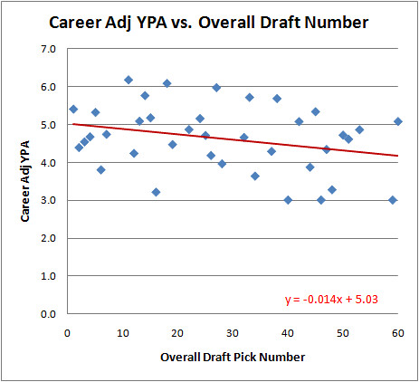
We can see a clear trend. Unsurprisingly, top picks would be expected to end up with better career passing stats than later picks. A linear regression estimates what the baseline expectation should be for each slot in the draft.
Next I calculated the 'Adj YPA above expected' for each QB. Now we can compare QBs who started their first year to those that didn’t, while holding “potential” equal.
But how do we define “started their first year?” How many starts qualifies--4, 5, 11? I don’t know, so let’s start by looking at the whole picture.
Results
We can use that baseline to compare each QB's career Adj YPA. Some QBs did better than expected given their draft slots and some did worse. We can now test if there is a connection between better than expected performance and the number of rookie year starts.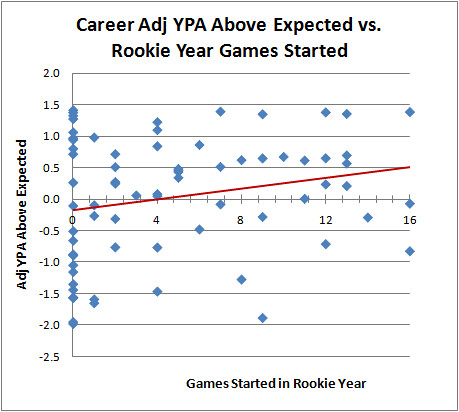
As it turns out, it appears that QBs with more rookie starts tend to enjoy greater career success, even accounting for draft order.
Some of you might have noticed that what I've really done here is a crude multivariate regression. Holding for draft order, I estimated the effect of games started. What if we just do the regression directly?
As expected we get a small negative effect with draft order. (The higher the pick number, the worse the expected stats.) The Games Started variable is positive and significant at p=0.03. The model as a whole has an r-squared of 0.15--small in absolute terms, but considerable given the highly random individual variance in QB careers.
But this is only one way of looking at whether a QB was a starter or not. What if we draw a line at say, 5 rookies starts--below 5 starts he's not a rookie starter and above it he is. The group of QBs with 5 or less starts averages -0.01 Adj YPA above expected, and the group with 6 or more starts averages +0.3 Adj YPA above expected. If we define it at zero starts, those with no rookie starts averaged -0.03 Adj YPA above expected, while those with at least one start averaged +0.02 starts above expected. In fact, no matter where I chose the endpoints of the groups, from 3 to 13 starts, the group with more starts outperforms the group with fewer starts by about 0.4 Adj YPA.
Conclusion
Does this mean teams should rush their rookies out to face the onslaught of NFL defenses to somehow make them better? I really doubt it. If I had to bet, I'd say that we simply haven't fully accounted for QB "potential" using draft order alone. I think the better QBs, those with the best chances of career success, often gain and maintain starting positions earlier.
But at the very least, we can say this: Given this analysis, there is no reason for a coach to arbitrarily keep a rookie QB on the bench. He should start his best QB, rookie or not, and not worry about incubating him under a ballcap on the sidelines. In the end, it should be the coach's qualitative judgment on the readiness of the player.
Here are the QBs and their stats I used for this article. (It's interesting just to see who the QBs are who exceeded expectations. There are some surprising names--Pennington and Batch at the top, for example. And Is Eli Manning really worse than David Carr? Wow.) You can sort the table by clicking on the column headers.Year Rnd Pick Name Team Adj YPA Exp Adj YPA Yr1 GS AdjYPA Abv Exp 2001 2 32 Drew Brees 
6.0 4.6 0 1.4 1981 2 33 Neil Lomax 
5.9 4.6 7 1.4 1998 1 1 Peyton Manning 
6.4 5.0 16 1.4 1998 2 60 Charlie Batch 
5.5 4.1 12 1.4 2004 1 4 Philip Rivers 
6.4 5.0 0 1.4 2004 1 11 Ben Roethlisberger 
6.2 4.9 13 1.3 1983 1 27 Dan Marino 
6.0 4.6 9 1.3 2000 1 18 Chad Pennington 
6.1 4.8 0 1.3 1999 1 11 Daunte Culpepper 
6.1 4.9 0 1.3 1984 2 38 Boomer Esiason 
5.7 4.5 4 1.2 1985 2 37 Randall Cunningham 
5.6 4.5 4 1.1 1983 1 24 Ken O'Brien 5.7 4.7 0 1.1 1995 2 45 Todd Collins 
5.3 4.4 1 1.0 1991 2 33 Brett Favre 
5.5 4.6 0 1.0 1983 1 14 Jim Kelly 5.8 4.8 0 0.9 1999 1 2 Donovan McNabb 5.9 5.0 6 0.9 1983 1 15 Tony Eason 
5.7 4.8 4 0.8 2003 1 1 Carson Palmer 5.8 5.0 0 0.8 1987 1 26 Jim Harbaugh 
5.4 4.7 0 0.7 1995 1 3 Steve McNair 
5.7 5.0 2 0.7 1996 2 42 Tony Banks 
5.1 4.4 13 0.7 1983 1 1 John Elway 5.7 5.0 10 0.7 1990 1 1 Jeff George 5.7 5.0 12 0.6 1997 2 42 Jake Plummer 5.1 4.4 9 0.6 2001 2 53 Quincy Carter 
4.9 4.3 8 0.6 1989 1 1 Troy Aikman 5.6 5.0 11 0.6 2003 1 7 Byron Leftwich 
5.5 4.9 13 0.6 1982 1 5 Jim McMahon 5.5 5.0 7 0.5 1995 2 60 Kordell Stewart 4.7 4.1 2 0.5 1986 1 3 Jim Everett 5.5 5.0 5 0.5 2002 1 32 Patrick Ramsey 
5.0 4.6 5 0.4 1999 2 50 Shaun King 
4.7 4.3 5 0.4 1989 2 51 Billy Joe Tolliver 4.6 4.3 5 0.3 2001 1 1 Michael Vick 5.3 5.0 2 0.3 2004 1 22 J.P. Losman 5.0 4.7 0 0.3 1987 1 13 Chris Miller 5.1 4.9 2 0.2 1993 1 1 Drew Bledsoe 5.3 5.0 12 0.2 1995 1 5 Kerry Collins 
5.2 5.0 13 0.2 1987 1 1 Vinny Testaverde 5.1 5.0 4 0.1 2003 1 22 Rex Grossman 4.8 4.7 3 0.1 1992 1 25 Tommy Maddox 
4.7 4.7 4 0.0 1986 2 47 Jack Trudeau 4.3 4.3 11 0.0 2002 1 1 David Carr 
5.0 5.0 16 -0.1 2004 1 1 Eli Manning 4.9 5.0 7 -0.1 1991 1 24 Todd Marinovich 
4.6 4.7 1 -0.1 1980 1 15 Marc Wilson 4.7 4.8 0 -0.1 1990 1 7 Andre Ware 4.7 4.9 1 -0.3 2003 1 19 Kyle Boller 
4.5 4.8 9 -0.3 1999 1 1 Tim Couch 
4.7 5.0 14 -0.3 1994 1 6 Trent Dilfer 4.6 5.0 2 -0.3 1999 1 12 Cade McNown 4.4 4.9 6 -0.5 1982 2 44 Oliver Luck 3.9 4.4 0 -0.5 1980 1 28 Mark Malone 4.0 4.6 0 -0.7 2002 1 3 Joey Harrington 4.3 5.0 12 -0.7 1986 1 12 Chuck Long 4.1 4.9 2 -0.8 1992 1 6 David Klingler 4.2 5.0 4 -0.8 1993 1 2 Rick Mirer 
4.2 5.0 16 -0.8 1983 1 7 Todd Blackledge 
4.1 4.9 0 -0.9 1991 2 34 Browning Nagle 3.6 4.5 0 -0.9 1982 2 48 Matt Kofler 3.3 4.3 0 -1.1 1994 1 3 Heath Shuler 3.7 5.0 8 -1.3 1992 2 46 Tony Sacca 3.0 4.4 0 -1.4 1992 2 40 Matt Blundin 3.0 4.4 0 -1.4 1999 1 3 Akili Smith 3.5 5.0 4 -1.5 1980 2 37 Gene Bradley 3.0 4.5 -1.5 2001 2 59 Marques Tuiasosopo 2.7 4.2 0 -1.5 1989 2 32 Mike Elkins 3.0 4.6 0 -1.6 1987 1 6 Kelly Stouffer 3.4 5.0 0 -1.6 1991 1 16 Dan McGwire 3.2 4.8 1 -1.6 1997 1 26 Jim Druckenmiller 
3.0 4.7 1 -1.7 1998 1 2 Ryan Leaf 3.1 5.0 9 -1.9 1981 1 6 Rich Campbell 
3.0 5.0 0 -2.0 1982 1 4 Art Schlichter 3.0 5.0 0 -2.0
Should Rookie QBs Start?

Live NHL Win Probability
 If you've been checking out the NBA win probability site, you've probably noticed a link for the NHL too. The probabilities are calculated based on the method I outlined in this post. The model now includes power plays, a unique and important factor in hockey.
Latest play descriptions are also included at each point in the graph, which is similar to how the football graphs will work in the fall. The most challenging part of whole project has been automatically adding notes to the graph where the goals were scored. They frequently overlap or overflow off the graph, and the logic of how to arrange them is far more challenging than you'd think.
I don't know much about hockey despite my frequent attendance at Capitals games in high school, and this has been a great way to look at the sport from a different perspective. I realize there aren't nearly as many hockey fans as football fans, but hey, a ten thousand Canadians can't be wrong...or however many Canadians there are. I missed that day at school.
The conference finals start today, so check it out. And if you're not interested in hockey, pass the word to your friends who are.
NHL Win Probability
Passing Predictability Part 2
 Here's a tip: If you author a sports research website, never start an article as "Part 1" unless you already have a Part 2 ready to go. Way back at the end of March I began looking at how predictability affects passing success. I looked at "10 yards to go" situations--1st and 10, 2nd and 10, and 3rd and 10 plays. Passes are least predictable on 1st down and most predictable on 3rd and long. With 10 yards to go, passes are called roughly half the time on 1st and 2nd down, but on 3rd and 10 passes are called 91% of the time.
Since then, I've been tinkering with my NBA and NHL in-game win probability sites. This post will officially tie the loose end that's been dangling since the NCAA Tournament.
In Part 1 of this article, we saw the average gain in each of these situations:Type 1st 2nd 3rd Total Pass 7.0 6.3 6.5 6.9 Run 4.2 4.4 6.9 4.3 Total 5.5 5.4 6.5 5.6
But there were several wrinkles in this analysis. First, there are interceptions to consider. Interceptions become much more probable on 3rd and 10.1st 2nd 3rd Total Int Rate 2.6 2.9 3.5 2.7
Combining Yards per Attempt and Interception rate yields Adjusted YPA, which is YPA with a -45 yd adjustment for every interception thrown.Type 1st 2nd 3rd Total Pass 5.9 5.0 4.9 5.6 Run 4.2 4.4 6.9 4.3
But there is still a problem. Adj YPA underestimates the drop off from 1st to 3rd down in passing effectiveness because defenses will allow gains, as long as they're not more than 9 yards. So we have to limit our observation to say the reduction in passing effectiveness due to predictability is likely at least 1 full adjusted yard per attempt.
Except that there's still another problem. There's a bias in the data because poor passing teams will face more 2nd & 10 and 3rd & 10 situations. So the 2nd and 3rd down numbers are lower than would be representative of the league as a whole. In other words, poor passing teams 'get more votes' in the analysis.
The solution is to give each team (or each team-year, actually) equal votes. Instead of averaging the gains for all 2nd and 10s for the entire league as a whole, I first averaged them by team-year, then averaged them by team.Stat 1st 2nd 3rd Total YPA 7.0 6.3 6.5 6.8 Int Rate 2.6 2.9 3.5 2.7 Adj YPA 5.8 5.0 4.9 5.6
As it turns out, the numbers are nearly (but not completely) identical using this method. The effect of the bias isn't very pronounced and we're left with the original estimate. Going from about 50% predictability to 90% predictability costs at least 1.0 Adj YPA.
Another notable observation is that although 1st &10 and 2nd & 10 have about the same run/pass balance of about 50%, passes on 1st and 10 are considerably more effective--5.8 vs 5.0 Adj YPA. I'd have to think that the difference may be largely due to play action.
Epic Bulls-Celtics Series
 If you haven’t been paying attention to this series you’re missing one of the most exciting 7-game series ever, even if it’s just the first round.
Going into Thursday night’s game, there were already 3 OT games and 1 last second buzzer-beater game. Then this happened: A 3OT potential elimination game that featured multiple furious comebacks for both teams and ultimately tied the series 3-3 with a 1-point win by Chicago. These two teams are as evenly matched as it gets. They square off for Game 7 tonight at 8.
Here are all 6 games of the series so far.
Compared to basketball or football, the hockey graphs aren't as compelling at first glance, at least during the game. But a quick look at a graph after the game tells a dramatic story you just won’t get with a box score. Below is Thursday night’s Game 1 between Chicago and Vancouver.
5-3? Well, that doesn’t sound terribly exciting. But check out what happened: 3-0 lead held until the third period. With 10 minutes left in the game, another goal, and with 5 min left another to tie it 3-3. Then Vancouver gets the game-winning goal with less than 2 min to go. Then in the final seconds, a garbage goal with the goalie pulled makes it 5-3.
You can check out the beta version of the hockey graphs for today's Caps-Penguins and Blackhawks-Canucks games. Power plays have not been factored in yet, but that's in progress, and it should be ready early next week.
NHL In-Game Win Probability
 I was at an NHL game the other night, and with the score 2-0 someone asked me, “So Mr. Win Probability, what’s the chance the Capitals win?” I was caught off guard, and after I choked out, “I…don’t…know…,” I experienced the horror that is not knowing the exact up-to-the-second win probability of a sporting contest. Don’t let this happen to you.
The anxiety and shame lasted for two days straight. I kept blaming myself and replaying the incident over and over in my head. The only way to cure my depression was to build a win probability model for NHL hockey.
Unlike my previous models for basketball and football which were empirically based, my hockey model is theoretical. In other words, instead of being based on a massive database of actual previous games, the probabilities are calculated based on a Poisson scoring distribution. The distribution is calculated using the average goals scored per minute in the 2008-9 NHL season. It’s an extension of the model I developed in this post.
Teams score an average of 2.79 goals per 60 minutes of regulation time, which is equal to 0.0465 goals per minute. A Poisson distribution based on that per-minute scoring rate and the time remaining in the game yields the probabilities of each team scoring each number of possible goals by the end of the game. Summing up all the probabilities of all the possible combinations of final scores gives the game’s win probability.
Here’s the graph:
There are a couple wrinkles to address. First, there are power plays. When a team as a man advantage on the ice, it’s much more likely to score. About one in five power plays results in a goal for the team with the advantage. Only about 2% of the time the short-handed team will score. So at the start of a power play, a rough approximation would put the win probability a little less than one fifth of the way toward the next best curve.
For example, if the score is 2-0 with 30 minutes remaining in the game, the win probability would normally be about 13% for the trailing team (the red line). But at the beginning of a power play, the trailing team’s win probability would jump about a fifth of the way up to the ‘down by 1’ line (blue). A rough approximation puts the new win probability at 16%. Then as the power play expires and there’s no score, the win probability would gradually return to the ‘down by 2’ line.
Second, there is the ‘end-game,’ when teams down by a goal will pull their goalie in favor of an additional skater. That would increase the win probability of the trailing team slightly, but only half as much as you might expect. They’d still only be buying an opportunity in overtime. But it could still be factored in. Before I do, I’d need some data on end-game goals.
One advantage of a theoretical approach over an empirical model is that team strength can be factored in far more easily. In an empirical model, when you divide up the data by various classes of team strength, the data is sliced into tiny fragments, usually with very small and unreliable sample sizes. Theoretical formula-based models don’t suffer from that problem. I can simply adjust the mean goals scored and goals allowed for any particular opponent, then rerun the model. The resulting model would be tailored to the specific match-up instead of a generic model for the league as a whole. Home ice advantage can be factored in with a similar approach.
Remember, WPD (Win Probability Dysfunction) can happen at any time, and it’s nothing to be ashamed of. Don't analyze win probability graphs if you take nitrates, often prescribed for chest pain, as this may cause a sudden, unsafe drop in blood pressure. Discuss your health with your doctor to ensure that you are healthy enough to view win probability graphs. If you experience chest pain, nausea, or any other discomforts during a sporting contest, seek immediate medical help. In the rare event of viewing win probability graphs more than 4 hours, seek immediate medical help to avoid long-term injury.
Live NHL win probability graphs now online.
Are Rookies Overpaid?
 I recently looked at what might explain why the top draft picks are paid disproportionately to their expected performance compared to later picks. But that doesn't address the larger issue--are rookies overpaid compared to their veteran counterparts?
A 2005 research paper called The Loser's Curse by economists Cade Massey and Richard Thaler tackled that question. In a nutshell, the paper compares rookie pay to the pay of a 6th-year veteran who could be expected to deliver the same performance as a rookie from each slot in the draft. (Performance is defined by a mix of measures including: being on a team roster, starts, and Pro Bowls.)
The conclusion of the paper is that team executives and scouts overpay for the top picks in the draft relative to the later picks, likely due to overconfidence in their ability to identify the best players. But what might surprise some readers is that rookies at every level of the draft are bargains compared to equivalently performing veterans.
This graph from the paper is the study's bottom line. The red 'compensation' line is the average annual pay for each draft pick. The blue 'performance' line is the salary a team would have to pay a 6-year veteran free agent for the same expected performance. The green 'surplus' line is the difference between the two pay levels.
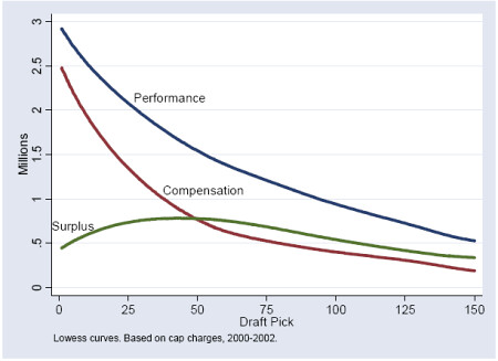
The surplus performance peaks shallowly at the bottom of the first round and through the second round. That's where teams get the biggest bang for the buck. But still, the surplus is strongly positive throughout the entire draft. According to Massey and Thaler, rookies are a bargain compared to veterans.
There's a good explanation why rookies would be underpaid. Veterans are known quantities while there is a tremendous amount of uncertainty with draft picks. Think of it this way--Peyton Manning has been to nine Pro Bowls and Ryan Leaf to zero, for an average of 4.5 between the two players. Four Pro Bowls--that's not bad. But would a GM pay more for a guaranteed 4.5 Pro-Bowl-type player or for a 50/50 shot between a total bust and Hall of Famer? Just about every modern economic and psychological theory tells us that people will pay a premium for the sure average.
Unfortunately, that's not an option in the draft. Peyton Leaf just doesn't exist. But 6-year veterans do, and GMs will be willing to pay a premium for the reduced uncertainty in performance.
One note of caution on the paper. The draft years studied were 2000-2002, and rookie salaries have increased substantially since then. But veteran salaries have too. The question is whether rookie pay increases have outpaced veteran pay increases since then. However, rookie pay would needed to have increased over 15-20% faster than veteran pay to change the conclusions of the paper.