Back Online, 2003 Added, and NBA Tonight

Comcast knocked out my server while I was out of the country on business earlier this week, so my apologies to everyone who linked to the NFL win probability archive. I'm pleased to report it's back up and running now.

I've added the 2003 season, so that covers every NFL game from 2003 through 2008. The 2000 through 2002 seasons will be added soon.

Also, don't miss the live NBA probability graph for game 4 of the finals tonight.

Two More Seasons Added

All games of the 2004 and 2005 NFL seasons are now charted and available. Win Probability graphs for the entire 2004 through 2008 seasons can be found at wp.advancednflstats.com/nflarchive.php.

Full 2006 Season Now Available

Another day, yet another year of games added. Win Probability graphs for the entire 2006, 2007, and 2008 seasons are now available at wp.advancednflstats.com/nflarchive.php.

Win Probability Graphs: 2007 Playoffs

+0.19 for Tyree’s catch.

+0.41 for the TD pass to Burress.

Sadly, no one will remember the 2-yd gain by Jacobs on 4th and 1 to keep the drive alive, but that play had a Win Probability Added (WPA) of +.21. If Tyree doesn’t make the catch, the drive is still alive--it was ‘only’ 3rd down. If Jacobs is stuffed—that’s all she wrote.

Of course, there’s no good way to quantify the style points for Tyree’s miraculous grab or Manning’s escape from the sack.

One of my major goals this off-season is to create win probability graphs for every NFL game since 2000. I'm starting with the 2007 playoffs, one of the most improbable championship runs ever. The New York Giants defied the odds in four consecutive games, never once favored to win. Yet somehow they slayed the dragon, the sport's most formidable offense in its history.

I'll be rolling out more than 2000 games over the next several days. Each graph has complete play-by-play descriptions. Just roll your cursor over the graph.

Also included are some new statistics. Comeback Factor (CBF) is simply the odds against the team that ultimately wins at their darkest moment. Excitement Index (EI) [boy, does that need a better name--I'll take suggestions] is how exciting the game was. Think of it as an EKG or Richter Scale for a game. It's the sum of all the movement in the graph. Blowouts are flat-lines and have relatively no movement, while close, high scoring games are the most exciting. Close, but low scoring games will be right behind.

In the play-by-play descriptions you might notice a stat labeled "LI." That's the Leverage Index, a concept borrowed from the sabermetric community and Tom Tango in particular. LI measures how crucial a particular game situation is toward the outcome. This should be an interesting new way to look at each play, and I'll explain it fully in a forthcoming article.

For now, keep the year menu on 2007. The playoff teams that year were the Colts, Pats, Giants, Jags, Titans, Steelers, Packers, Seahawks, Redskins, Cowboys, Bucs, and Chargers.

There are still a few hiccups with the graphs, usually due to errors in the NFL gamebooks I use to create them. Comments and suggestions are more than welcome.

wp.advancednflstats.com/nflarchive.php

Injury Rates and An Extended Season

At the recent owners meeting, the NFL disseminated a study that concluded an increase in the season schedule from 16 to 18 games would not increase injury rates. The report caught a lot of criticism as a halfhearted attempt to obscure the toll a longer season would take on the players. Judy Battista of the New York Times and Mike Reiss of the Boston Globe both point to flaws in the study.

But I suspect there is a fundamental misunderstanding about what the report says and how it's being interpreted. All I really know about the report is that it says, "the NFL's injury rate doesn't increase at the end of the season." There is no doubt a longer season would result in more total injuries. The bigger question is how many more injuries--does the injury rate itself increase?

Much of the criticism of the study focuses on the use of team injury reports, well known for their deceptive omissions. In an excellent article, Bill Barnwell at Football Outsiders found an additional flaw in the study. It left out players who go on the IR. Before you consider players on the IR, it appears that the injury rate peaks at week 10 before it decreases for the remainder of the season. Barnwell explains why this isn't really the case.

Since team injury reports are notoriously unreliable, the best information is actual games missed. Thankfuly, Barnwell provides that data in his article, and it's very interesting stuff. When you factor in the IR, the number of games missed climbs steadily. He concludes, "the data looks totally different, and in a bad way for the NFL..."

The way I see it, however, is that the NFL report is right, no matter what the intent was of its authors. There is no increase in injury rates toward the end of the season. The injury rate is effectively linear. Of course, as the season wears on, the number of players unable to play due to injury will accumulate, creating an upward climbing injury total. Once you go on the IR, you don't come off. This cuts to the heart of the debate about whether players become increasingly susceptible to injury as the season, along with the number of cuts and collisions, wears on.

Here is a graph of the data included in the Barnwell article.


The blue line is the games missed by roster players (those not on the IR). Except for the uptick on the final week, when playoff bound players nurse their wounds and everyone else has their bags packed for the Caribbean, it's very steady. The green line is the number of games missed by IR or physically unable to perform (PUP) players. Note how its slope steadily increases. The red line is the combination of the injured roster players and IR/PUP players.

Here's what I take away from this data. Players on the IR increase at a (very) slightly exponential rate--specifically it's:

#IR = 0.006w² + 0.1w + 1.6, where w=week.

That .006 term is extremely small, and when combined with the negative camber of the blue line, results in a very linear total, (especially when week 17 is thrown out, although you don't need to.) [Note: By the way, the slight non-linearity of the increase is evidence, however tiny, for the notion that players become more susceptible to injury as they endure the season.]

Ultimately, the total number of players who miss games due to injury is indistinguishable from a linear line (r-squared of .97). Its increase is exclusively due to players going on the IR, which is a one-way check valve.

So will there be more players missing games at the end of the season if the NFL adds two more games? Of course. But it won't be Iwo Jima out there. No explosion of wounded players with "cascading" injuries. It will be a demanding, grueling, even cruel extra two games for the players, but it would barely be noticeable to the fan and to the game itself. I suspect that's what the NFL report is trying to spell out. Even counting the uptick in the final week, each team would average an extra half a missed player by a potential week 19.

Personally, I'm against lengthening the season for a lot of reasons. The nerdiest is that there is a mathematical elegance to 2 conferences, 4 teams per division, 8 divisions, 16 games, 32 teams, and 256 games per season. Please, no 17th game or 33rd team--I'd have to redo all my algorithms and equations! Actually, I just think 16 is plenty. The fewer the number of games, the more unpredictable the season, and I like that.

Michael Vick Was a Better QB Than You Think

Before Michael Vick's run-in with the law, he was widely considered an exciting and elusive quarterback with below-average throwing ability. Usually, his poor completion percentage is cited as evidence of his lackluster passing ability. It seems that reputation is still with him. Case in point is this excerpt from Peter King's most recent post:

Well, as a quarterback, Vick was decidedly mediocre in his four full seasons starting for the Falcons. His completion percentages when he started at least 15 games -- 54.9, 56.4, 55.3 and 52.6 -- were poor; he had 36 fumbles and 38 interceptions in his last 46 starts.

One thing is certain--Vick is (or was) an unconventional QB. He was a breakaway runner without peer, and the normal rules of quarterbacking don't apply. The vast majority of Vick's 529 career runs were scrambles on pass plays. When a conventional QB progresses through his reads, he looks at WR#1, WR#2, TE, and then dumps off to a RB. But Vick, on the other hand, doesn't bother with the dump off. He is the dump off.

Most of Vick's 52 running yards per game can really be credited as passing yards. They were yards gained on pass plays in passing situations. He averaged 7.1 yards per run. Compare that to the NFL's 5.0 average net passing yards per attempt and 4.1 rushing yards per attempt. And remember, there is never a risk of interception if he tucks the ball and runs. If you factor in his sacks into his rushing average, it becomes 5.1 net yards per run, which is still good. But if we do that, it would make his net passing yards per attempt much higher. After all, we can only count his sack yards against him once. Otherwise, it's double jeopardy.

So Vick's pass completion stats aren't padded by lots of rinky-dinky dump offs. David Carr actually led the NFL in completion percentage in 2006 with a gaudy 68.3%, only to lose his job the following off-season (to Vick's backup nonetheless).

To get an idea of how deep Vick was throwing compared to his league counterparts, we can look at yards per completion. In 2006, the most recent year Vick played, the league's other top 30 QBs averaged 11.4 yards per completion, while Vick averaged 12.1.

Vick's receiver corps in Atlanta was never known as particularly talented. If we remove receiver YAC from the equation, the numbers are even more favorable for Vick. His Air Yards, the yards a complete pass travels in the air forward of the line of scrimmage, is impressive. The top 30 other QBs in 2006 averaged 6.3 Air Yds per completion, while Vick averaged 7.7.

Yes, his interception and fumble rates are higher than you'd like, but those too should be considered in the context of the depth of his throws and the frequency with which he runs. So although Vick's passing stats, especially completion percentage, appear sub-par, that should be expected, and they are somewhat offset by greater gains for each completion. I'm not claiming he's great, or even above average, just better than his conventional stats suggest.

Are NFL Coaches Too Timid?

Risk is at the heart of football strategy. Aggressive, risky gameplans should result in boom-or-bust high-variance outcomes, sometimes scoring lots of points but sometimes scoring very few. Conservative gameplans result in relatively consistent low-variance outcomes. Teams would more likely score close to their average score.

In this post, I’ll look at what high and low variance strategies would look like in terms of point totals and how they affect each team’s chances of winning. I’ll also compare the theoretical strategies to the actual distributions in the NFL. We'll see why NFL coaches should be more aggressive when they're the underdog.

High Variance Strategy in Basketball

Some time ago, I came across an article posted by basketball researcher Dean Oliver that analyzed high and low variance strategies for the NBA. Oliver calculated the win probability of each opponent according to the mean and standard deviation (SD) of each team’s scoring tendencies. SD represents the degree of variance. The more aggressive and riskier the strategy, the higher the SD will be. For example, a basketball team that shoots lots of 3-pointers would have a high variance.

The key to accurately modeling basketball is realizing that each team’s score is correlated with that of its opponent. The pace of a basketball game ties each team’s score together, and there is a high level of covariance. When one team scores a high number of points, the other team will tend to score more too. Game scores are interdependent.

In Football

Recently the Smart Football blog illustrated the advantage of high variance strategies for underdogs. A high variance strategy increases an underdog’s chances of winning but comes with the cost of also increasing its chances of being blown out.

In the NFL as a whole, visiting teams average about 19 points with a SD of 10 points while home teams average about 23 points with a SD of 10 points. But unlike basketball, football opponent scores are negatively correlated. This makes intuitive sense because the better one team does, the worse the other should do. If one team gets lots of first downs and doesn’t commit turnovers, its opponent will usually start drives with poor field position, and vice versa. The covariance between NFL opponent scores is -1.9 points-squared.

If NFL scores were normally distributed, this is what the typical score distribution would look like. The visitor scores are in red and the home scores are in blue.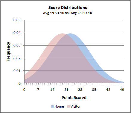


We can calculate each team's chances of winning by summing all the probabilities with these distributions and factor in the covariance using Dean Oliver’s method. This estimates that the home team wins 56.5% of the time, which happens to be exactly the NFL actual home field advantage.

Disclaimer

There’s one problem. NFL scores are not normally distributed, primarily due to its unique scoring, which typically comes in chunks of 3 or 7. Here is what the actual distribution of scores looks like.


The good news is, if we group the scores into bins of 7 points, we get a quasi-normal distribution. (Technically, it may be more of a gamma or Poisson distribution.) I’m going to stick with normal distributions to simplify the math and to better illustrate the concepts I want to convey.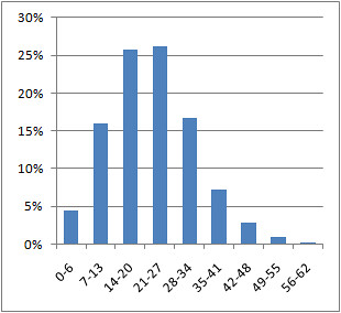



Demonstration

Here’s why underdogs should play aggressive and risky gameplans. Take an example where one team is a 7-point favorite over its underdog opponent. Say the favorite would average 24 points and the underdog would average 17 points. With a SD of 10 points for each team, the underdog upsets the favorite 31.5% of the time. The favorite’s scoring distribution is blue and the underdog’s is red.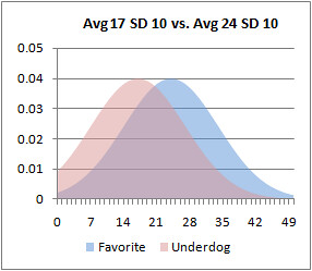


But if the underdog plays a more aggressive high-variance strategy, increasing its SD to 15 points, it would upset the favorite 35.3% of the time.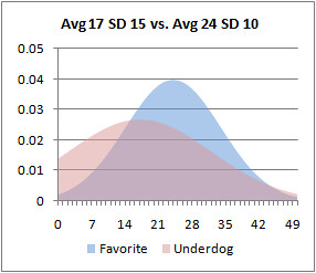


Note that I haven’t increased the underdog’s average score in any way, just its variance. The increase in its chance of winning results due to more of its probability mass moving to the right of the favorite’s mean score of 24. In fact, the higher the variance, the wider the probability mass will be spread. Consequently, more mass will be to right side of the favorite’s average score. But more mass will also be to the left, meaning there is a higher risk of an embarrassing blowout.

Even if employing a high-variance strategy is non-optimum, it can still help an underdog. In other words, even if an aggressive gameplan results in an overall reduction in average points scored, it often still results in a better chance of winning.

The next graph plots the scoring distributions of just such a scenario. Like before, the favorite’s average score is 24 with a SD of 10. But this time the underdog’s average is reduced from 17 to 16. The increase in variance still results in a slightly better chance of winning despite its overall reduction in average points scored. In this case, it's 33.2% for the underdog.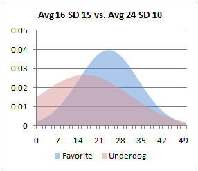


What about the favorite? Should it increase its variance in response to an aggressive underdog? No. Ideally it should play as consistently as possible. The lower the variance the better for the favorite. The next example shows a favorite playing a low-variance game with an average of 24 points and a SD of 5 points. The underdog is playing conventionally with a 17 point average and 10 point SD. The result is an increase in the favorite’s chances of winning from 69.5% in the original example to 73.0%.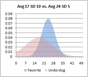


And if the underdog plays an aggressive high-variance game, the low-variance strategy is still better for the favorite. In this case the favorite still improves its chances of winning from 64.7% to 67.8%.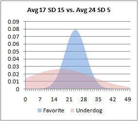


In Practice

So what does any of this mean in the real world? Simply put, to win more often underdogs should employ a high-variance strategy from the beginning of the game. It shouldn’t wait until the 4th quarter and become desperate. Go for it on 4th and short, run trick plays, throw deep, and blitz more often. Roll the dice from the get-go.

The real question is, what is the optimum level of risk? I’m not sure, but I do know NFL coaches are operating far from it.

Looking at games from the ’02 through ’06 seasons (a total of 1280), underdogs do not increase their variance. For example, for games in which the point spread is between 6 and 7.5 points, the underdog’s SD is 9.8 points, slightly less than the overall league average. Ideally, it should be higher. The favorite’s SD is 10.4 points when ideally it should be lower.

The table below lists the SDs of points scored for the favorite and underdog according to the most common point spreads.

Spread	Favorite SD	Underdog SD
0 - 1.5	9.6	10.5
2 - 3.5	9.8	9.4
6 - 7.5	10.4	9.8
10 - 11.5	10.5	8.7

If anything, there appears to be slight trends in the exactly wrong directions. The bigger the spread, the smaller the underdog’s variance and the bigger the favorite’s variance. It appears underdogs may get less aggressive while favorites may get more aggressive.

Conclusions

This is more evidence coaches do not coach to maximize their team’s chances of winning. My theory is coaches are delaying elimination until the latest point in the game—that is, trying to “stay in the game” for as long as possible. Underdog coaches minimize risk all game long hoping for a miracle along the way. They seem to be reducing the chances of being blown out, but this is not consistent with giving their team the best chance to win.

But if you think about it, this kind of approach might be good for the NFL as a whole. It keeps games entertaining as long as possible, and keeps viewers tuned in.

Coaches of favored teams could be accused of the same crime. They might be playing with too much variance. But there is certainly a limit to just how consistent a team can be, no matter how hard it tries. There will always be random variation in team performance. I suspect a SD of 10 points may be near that limit, and that coaches of both favorites and underdogs simply play the least risky game they can consistent with accepted conventions.

Thoughts on the Apparent Unimportance of Run Defense

John Morgan of the Seahawks blog Fieldgulls.com asked me recently about why run defense appears relatively less important in terms of winning than do other facets of the game. John writes:

You state defensive rushing yards per attempt allowed is the least important component to winning, but I wonder if that factors in game situation. Losing teams are likely to reduce their yards per attempt allowed when winning teams are running out the clock.

John makes a good point, and indeed the team-stat regression model I used when I made that conclusion did not take game situation into account. John goes on to point out that teams that are already behind may face a large number of predictable run-out-the-clock runs, which would make their run defense appear better. Plus, the game theory aspects of running and passing should enable a good run defense to make stopping the pass easier.

I think this is an interesting point, and I soon should be able to test how much late-game runs affect a team’s overall defensive efficiency after some improvements to my play-by-play database. A preliminary look indicates it probably doesn’t make much of a difference. Still, I think John raises good points about the game theory aspect and predictability.

In theory, good a run defense should make a pass defense better. And the stats suggest it does. The correlation between defensive running efficiency and passing efficiency is 0.20. Some of that correlation has to do with the fact that superior defensive athletes are superior against both the run and the pass. But some of it should also be due to the game theory aspect.

(In comparison, offensive running and passing efficiency correlate at 0.13. I think the difference is that there is a lot more variance in offensive passing than in other facets due to the focus on a single player’s ability. The quarterback’s contribution is so critical to passing in ways that aren’t applicable to the other aspects.)

According to game theory principals, defensive running and passing would only be equally important if offenses and defenses were operating at the game equilibrium point-- that is, they’re playing the optimum mix of passing and running. But I think they might not be.

My theory is that this may be why run defense appears so unimportant. Say teams are not operating at the game equilibrium, and passing is, on balance, a more lucrative strategy than running. In other words, there really is a considerable passing premium where the payoff for a pass is generally higher than a run, all things considered.

Having a good run defense would therefore be somewhat self-defeating. Take the 2007 Vikings defense that gave up only 3.1 yards per run (good) but 7.0 yards per pass (bad). Facing such a solid run defense, a good offensive coordinator is forced to pass more…which would be a far more effective thing to do in the first place, especially against a relatively weak pass defense. A team like the 2007 Vikings would essentially be forcing their opponent to unwittingly play a more efficient and effective strategy, all the while exploiting their own weakness.