by Ben Zauzmer. Ben is a junior majoring in Applied Math at Harvard University and is a member of the Harvard Sports Analysis Collective. This article was originally published at harvardsportsanalysis.org.
In 2012, the NFL created new overtime rules designed to make the game fairer. The league switched from a sudden death setup to an arrangement that allows both teams to have a chance at scoring, unless the first team to receive scores a touchdown. Even with this change, it would seem that a coach should still always elect to receive if he wins the coin toss at the start of overtime, since an opening touchdown drive wins the game.
However, earlier this year, for the first time under the new rules, a coach made exactly the opposite decision. Bill Belichick, the three-time Super Bowl-winning coach of the New England Patriots, made the gutsy call to kick at the start of overtime. Many considered the main factor behind this decision to be the heavy winds at Gillette Stadium (if a team defers the choice of kicking or receiving, it may choose which direction to face). However, kicking first may also give a team better field position on offense and may actually benefit teams with strong defenses.
To calculate which strategy coaches should prefer, we will model NFL overtime as a Markov Chain. We will define our states as the set of possible point differentials, from the perspective of the team that receives the opening kickoff, in overtime: -6, -3, -2, 0, 2, 3, 6. This model inherently assumes that state-to-state probabilities are not conditional, and that the probability of the score differential being 5 or 9 – both technically possible under the new rules – is negligible.
We will let be the transition matrix for the receiving team’s first offensive possession, be the receiving team’s first defensive possession, be every subsequent receiving team offensive drive, and be every subsequent receiving team defensive drive. The first row/column of each matrix represents the receiving team at a -6 scoring difference, and so on until the last row/column is the receiving team at a +6 scoring difference.
The matrices have the following forms:
Note that every overtime starts off with the score tied, so the initial probability distribution is:

We proceed recursively, alternating between which teams has the ball.

For even integers :

For odd integers :

After a kickoff, drives end with the following frequencies (all stats from www.pro-football-reference.com):
Defensive TD: .020
Safety: .001
No Score: .661
FG: .118
TD: .200
After a non-kickoff, drives end with the following frequencies:
Defensive TD: .017
Safety: .004
No Score: .583
FG: .175
TD: .221
If overtime were allowed to go on forever, as in the NFL playoffs, the stationary probability distribution would be:

This is a reasonable estimate for the probability of the game ending in any one of these potential states. For instance, the probability that the team which first received the ball in overtime losing by 6 is 25.6%.
Then, the probability of the receiving team losing is (decimals are rounded):
.256 + .205 + .004 = .464
The probability of the receiving team winning is:
.004 + .179 + .353 = .536
The probability of a tie is 0, which makes sense because after an infinite number of drives, the probability of nobody scoring approaches 0. So, in this simple model, the team that wins the opening coin toss should always choose to receive.
For regular season play, we need to take into account average time per possession. In 2013, this is 2:34, meaning we expect only about 3 drives per team before the 15-minute overtime period ends in a tie. Therefore, a more realistic probability distribution is:

Using identical sums as the infinite overtime model, the probability of the receiving team losing is .446, the probability of the receiving team winning is .507, and the probability of a tie is .047.
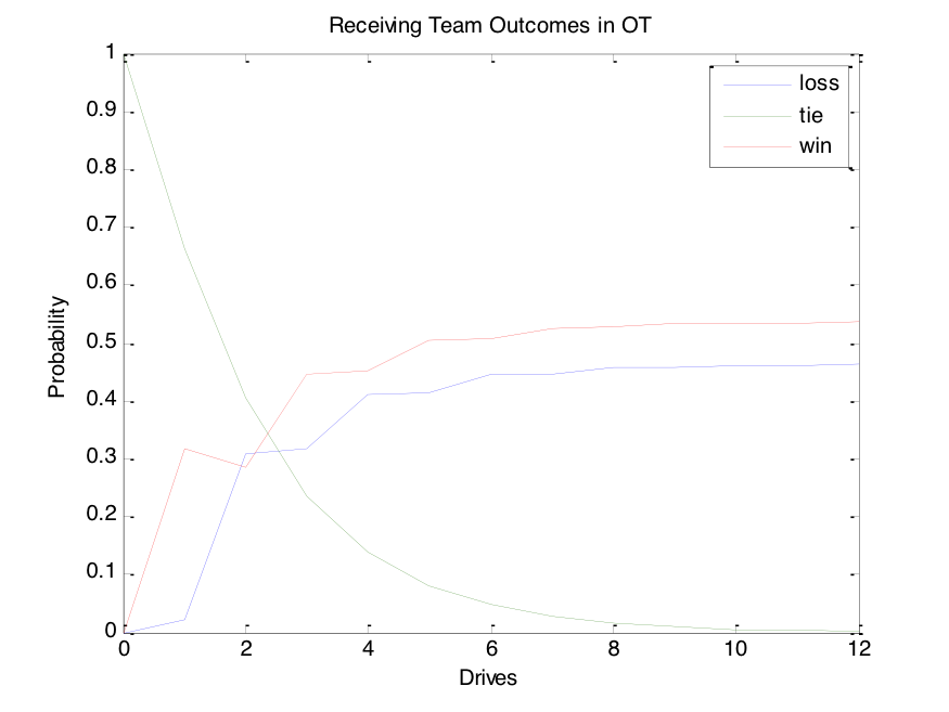
The count of six drives per overtime period is only an estimate. Therefore, it is more useful to consider probabilities for each team winning and tying over a range of possible numbers of drives.
The red (receiving team wins) and blue (receiving team loses) curves move further apart on odd numbers and closer together on even numbers. This makes sense, because after an odd number of drives, the receiving team has the unfair advantage of having had an extra drive to try and score. There is technically also a chance for the defense to score on any drive through a safety or a defensive touchdown, but the probabilities are not nearly as high as those for the offense scoring a field goal or touchdown. The red and blue curves eventually reach a steady state, which is calculated in our earlier section on infinite overtime.
There is one time-step (after each team has had exactly one drive) in which it is better to be the kicking team. If the overtime lasts two drives – that is, each side get the ball once – the kicking team has a slightly higher probability of winning. For any other number of drives, it is better to be the receiving team.
The next step is to include team-specific data. A relatively good offensive team would rather get the ball first in an attempt to score and win before the other side can get the ball. A relatively good defensive team might prefer to kick off to start OT, in the hopes they can stop the opposing offense first.
Instead of using league average for all of the constants, we will now use the average of one side’s offense and the other side’s defense. For instance, if the Eagles are playing the Cowboys, the probability of the Eagles’ offense scoring a touchdown against the Cowboys’ defense will be estimated as the Eagles’ offense touchdown frequency and the Cowboys’ defense touchdown allowed frequency. Instead of using 2:34 as the average drive length, we will take the average of the mean drive lengths for each team in question.
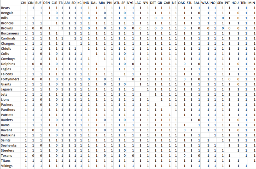
To put it all together, the following is a chart of every possible NFL matchup. A 1 means the team in that row would prefer to receive against the team in that column. A 0 means they would prefer to kick.

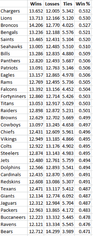
An interesting follow-up question is which teams are best equipped for overtime. We will assume that each side has perfect information, meaning they know where all the 0s and 1s are placed in the above table and always make the right decision on whether to kick or receive. Then, since the deciding team is chosen by coin toss, there is a 50% chance of each occurring in any game. We will simulate a 31-game “season” for each team, where everybody plays everybody else exactly once, and all games go to overtime.
The final expected standings are as follows:
In general, better teams do better and worse teams do worse, but it is not a strict correlation and there is not much separation between the good teams and the bad. This shows how much variance there is in an overtime when one score is usually enough to win the game. In the regular season, albeit with fewer games (teams play 16 games per year, not 31), there is far more of a range of winning percentages. The reason is that most games do not go to overtime, and are therefore decided by many scores, not just one. This allows the better team to win more often than a modified sudden death overtime setup does.
Of course, there are other factors beyond overall team averages to account for. If a key player, such as a placekicker, is injured, that would affect the relative strengths and weaknesses of each team going into overtime. If there is heavy wind in one direction, the coach might prefer to defer the decision on kicking or receiving in favor of choosing which direction his team will drive. If he feels one team is better conditioned than the other, he might have some foreknowledge of how many drives will take place, since players are likely to get tired when asked to play more than their usual 60 minutes of football. With that said, coaches need to consider the data in advance of each game, just in case they end up with a difficult and sure-to-be-scrutinized decision if the game winds up tied at the end of regulation.


Isn't using the 2:34 TOP per drive useless for Overtime since teams can choose to speed it up late or milk the clock in OT? Why not use the observed overtime TOP?
It would be interesting to see, instead of just 1 to receive and 0 to defer, by how big a margin the decision to receive and defer is favoured as this would then be impacted by the other factors you mention which could affect the decision. If you would elect to receive by a very big margin, for instance, it may be that you would not be all that bothered by the wind conditions for example.
I did a similar analysis on this site last year, with similar results (http://www.advancednflstats.com/2012/12/markov-model-of-overtime.html) but the main qualifications for both that and this is that behavior in OT is different than regulation (in particular after the initial 0-0 state). So those drive-ending probabilities based on regular season data won't be great (and there is not new enough OT data yet to really be confident). The TOP issue anonymous raises above is also a significant issue - underdogs would definitely prefer to use as much time as possible to increase the probability of a tie.
Definitely a very interesting topic though, and will become easier to study as data increases.
The biggest problem here is that the A2 matrix is going to be very different in the -3 state, where the trailing team is playing 4 down football. My guess is that other drives also have different transition matrices, too. The opening drive has a very different FG/TD payoff, so one would expect that the results would differ also. After the first drive, FGs become as valuable as TDs, so I would expect the results to differ as well. It's hard to guess what the results are, but to guesstimate, you could look at all OT drives before the rule change to get an idea.